Abstract
Substance use disorders are characterized by reduced control over the quantity and frequency of psychoactive substance use and impairments in social and occupational functioning. They are associated with poor treatment compliance and high rates of relapse. Identification of neural susceptibility biomarkers that index risk for developing a substance use disorder can facilitate earlier identification and treatment. Here, we aimed to identify the neurobiological correlates of substance use frequency and severity amongst a sample of 1,200 (652 females) participants aged 22–37 years from the Human Connectome Project. Substance use behaviour across eight classes (alcohol, tobacco, marijuana, sedatives, hallucinogens, cocaine, stimulants, opiates) was measured using the Semi-Structured Assessment for the Genetics of Alcoholism. We explored the latent organization of substance use behaviour using a combination of exploratory structural equation modelling, latent class analysis, and factor mixture modelling to reveal a unidimensional continuum of substance use behaviour. Participants could be rank ordered along a unitary severity spectrum encompassing frequency of use of all eight substance classes, with factor score estimates generated to represent each participant’s substance use severity. Factor score estimates and delay discounting scores were compared with functional connectivity in 650 participants with imaging data using the Network-based Statistic. This neuroimaging cohort excludes participants aged 31 and over. We identified brain regions and connections correlated with impulsive decision-making and poly-substance use, with the medial orbitofrontal, lateral prefrontal and posterior parietal cortices emerging as key hubs. Functional connectivity of these networks could serve as susceptibility biomarkers for substance use disorders, informing earlier identification and treatment.
1. Background
Substance use disorders (SUDs) describe a constellation of symptoms characterized by continuing use of one or more intoxicating substances despite significant negative consequences (American Psychiatric Association, 2013). Symptoms include reduced control over the quantity and frequency of use, hazardous patterns of consumption, and accompanying impairments in social and occupational functioning (American Psychiatric Association, 2013). Prevalence of SUDs is estimated as high as 12% for alcohol and 2–3% for illicit drugs (Merikangas & McClair, 2012). Additionally, SUDs are associated with significant social harms and often poor treatment response characterized by poor compliance and high rates of relapse (Miller, 1996). Thus, there is a need for earlier identification and treatment of SUDs (Yücel et al., 2019). For example, the term ‘preaddiction’ has been coined to refer to mild to moderate SUDs that have not yet progressed to severe levels (‘addiction’) and may represent a critical treatment window (McLellan et al., 2022). However, there are no objective biological assessments available for evaluating risk for SUD.
A central aim of contemporary psychiatric research is the identification of susceptibility biomarkers - measurable biological characteristics that index liability for psychiatric illness (Beauchaine, 2009, Califf, 2018, Singh and Rose, 2009). Susceptibility biomarkers hold great promise for improving mental health treatment through earlier identification of psychopathology (Cook, 2008). Over the past decade, there has been an interest in incorporating neurobiological findings into the diagnosis and treatment of mental disorders (Cuthbert and Insel, 2013, Hyman, 2007). Shared neurobiology emerged as a key validator introduced by the Diagnostic and Statistical Manual of Mental Disorders – Fifth Edition (DSM-5) Task Force Study Group for exploring the proposed reorganization of diagnostic categories, including SUDs, into metastructures based on comorbidity, common etiology, course of illness, treatment response, and shared neural substrates (Andrews et al., 2009).
Research based on traditional psychiatric nosology has conspicuously failed to yield robust evidence of the neurobiological mechanisms underlying psychopathology (Hyman, 2007, Jablensky, 2016, Maj, 2014). To circumvent these limitations, psychiatric research is transitioning away from traditional categorizations of mental disorders as discrete diagnostic entities towards empirically-based, dimensional models of psychopathology, such as the Research Domain Criteria (RDoC) (Cuthbert, 2014). Dimensional models are better positioned to identify shared aetiological mechanisms of psychiatric disorders by capturing phenotypic variation across the full spectrum of symptom severity (Cuthbert, 2014, Patrick et al., 2013). A wealth of evidence indicates that substance use problems constitute a dimensional continuum in the population with no natural demarcation point designating problematic from non-problematic use (Kraemer et al., 2004, Miettunen et al., 2016). There is also evidence to suggest that partially discrete models with clinically relevant subgroups embedded within a dimensional continuum is the most accurate characterization of some forms of psychopathology (Helzer et al., 2006, Krueger and Bezdjian, 2009). In particular, clinical phenomena such as substance use measured in non-clinical samples are characterized by ‘zero-inflation’, in which there are a large number of individuals with little-to-no symptoms (B. Muthén, 2006). Hybrid models, combining features of categorical and dimensional psychopathology, are a promising alternative approach to psychiatric research (Feczko et al., 2019, Krueger et al., 2018, Krueger and Bezdjian, 2009). Factor mixture modelling (FMM) is a type of latent variable analysis that combines the common factor modelling approach with latent class analysis (LCA) (Borsboom et al., 2016, Clark et al., 2013).
The approach can be used for identifying discrete, latent (i.e., not directly observed) classes or clinical subtypes embedded within multivariate dimensional data, including zero-inflation (Borsboom et al., 2016). Specification of a priori subtypes provides a natural demarcation in multivariate space that substantially reduce the dimensionality of the data and renders analysis of complex phenotypic data more tractable (Feczko et al., 2019). Hybrid models, such as FMM, may be important for identifying clinically meaningful subtypes with implications for informing earlier targeted interventions for those with ‘preaddiction’.
In terms of what this proposed continuum of substance use frequency reflects neurobiologically, there are several possibilities. Functional neuroimaging analysis of human decision-making has converged on a collection of cortical and subcortical brain regions involved in value-setting and intertemporal choice, (the preferential selection of rewards based on both magnitude and delay until obtainment) (Hamilton et al., 2015): the Valuation (VS), Executive Control (ECS) and Prospection (PS) Systems. The VS (ventromedial prefrontal cortex, nucleus accumbens, amygdala and the posterior cingulate cortex) encodes the subjective values of various options during decision-making (Kable and Glimcher, 2007, Kable and Glimcher, 2010, Laurent et al., 2015, Peters and Buchel, 2010b), as well as generating goal-directed drug-seeking urges (Berridge, 2012, Leyton and Vezina, 2014, Steketee and Kalivas, 2011, Wolf, 2016). The ECS (dorsal anterior cingulate cortex, lateral prefrontal cortex and posterior parietal cortex) inhibits impulsive responses (van den Bos & McClure, 2013) via the incorporation of past outcomes and future goals (Kim et al., 2009, Sutton and Barto, 1998). The PS (dorsomedial prefrontal cortex, precuneus and medial temporal lobe) is activated during episodic memory recall or simulation of potential future scenarios (Schacter et al., 2007) involving drug use behaviour (Fang et al., 2021, Karch et al., 2015) and is thought to be associated with a preference for delayed rewards (Lempert et al., 2019). It is worth noting that regions of the VS (parts of the medial prefrontal and posterior cingulate cortices) and PS (middle temporal lobe, middle prefrontal cortex and precuneus) overlap with those recruited by the default mode network (Alshelh et al., 2018). However, the terms VS and PS are used for clarity as they better define the roles played by these regions with respect to value-based decision-making and delay discounting.
During dependency, addictive substances may enable the achievement of desired states (e.g., euphoria or pain relief). This is underpinned by the activation of, and interactions between, the VS, ECS and PS (Loganathan & Ho, 2021). The instrumental pursuit of addictive drugs can then lead to the development of choice impulsivity (Oberlin et al., 2021), the preferential selection of smaller, more immediate rewards over larger, delayed rewards (Hamilton et al., 2015). Research indicates a significant relationship between delay discounting (a measure of choice impulsivity) and substance use behaviour in both adolescents and adults (Audrain-McGovern et al., 2009, Khurana et al., 2013, Khurana et al., 2017). A recent systematic review of task-based connectivity correlates with delay discounting behaviour (Owens et al., 2019) highlighted studies which showed positive correlation between functional connectivity and stronger delay discounting (i.e. greater impulsive choice) (Clewett et al., 2014, Contreras-Rodriguez et al., 2015) among cocaine and tobacco dependents. Particularly, connections within the fronto-parietal network (i.e., lateral prefrontal and posterior parietal cortices) were positively-correlated with steeper discounting among tobacco-smokers (Clewett et al., 2014). Stronger connections were observed between the caudate and anterior cingulate cortex in correlation with steeper discounting in cocaine dependents (Contreras-Rodriguez et al., 2015). While these studies must be praised for linking task-based delay discounting data with functional connectivity among substance dependents, an over-arching limitation remains the focus on a single substance rather than considering poly-substance use behaviour.
Turning the focus to resting-state fMRI studies, it has been observed that under normal circumstances, the interaction between VS and ECS is balanced, regulating impulsivity by incorporating phases of well-deliberated, disciplined thought and action (Dalley et al., 2011, Xie et al., 2014; T. Zhai et al., 2015). However, during dependency, VS activation appears to no longer be counterbalanced by the ECS, biasing decision-making towards the pursuit of drugs (Xie et al., 2014; T. Zhai et al., 2015). Interestingly, the PS has been implicated in reducing impulsive choice (Peters & Buchel, 2010a) by counteracting the growing predisposition towards more impulsive choices (VS) and concomitant reduced cognitive control (ECS) (Li et al., 2015, Liu et al., 2018, Verdejo-Garcia and Bechara, 2009, Xie et al., 2011; T.-Y. Zhai et al., 2014; T. Zhai et al., 2015). Participants living with cocaine dependence showed significant activation in the middle and superior frontal cortices, anterior cingulate, striatum and midbrain during a loss-chase task (Worhunsky et al., 2017), suggesting an integration of signals from regions of the VS, ECS and PS that contribute to choice impulsivity. These findings indicate that increased participation of valuation and decision-making regions may be required when losing gambles. Connectivity within the orbitofrontal cortex and amygdala (both VS) during cocaine dependency suggests that increased value has been placed on this stimulant as a reward of choice (Contreras-Rodríguez et al., 2016). Additionally, connections between the nucleus accumbens (VS) and parts of the dorsolateral prefrontal cortex and dorsal anterior cingulate cortex (ECS) were weakened during dependency, reflecting reduced levels of behavioural control (Berlingeri et al., 2017, Motzkin et al., 2014). These individuals also expressed increased connectivity between regions of the anterior cingulate cortex and dorsolateral prefrontal cortex (both ECS) with middle temporal and superior frontal gyri (both PS), indicating increased cognitive resources required to implement cognitive control (Camchong et al., 2011). Among alcohol abstainers, an inverse activation synchronicity between the nucleus accumbens (VS) and dorsolateral prefrontal cortex (ECS) suggests that increased resources are allocated to regulate behaviour away from alcohol consumption. Furthermore, reduced activation of the nucleus accumbens reflects restricted reward processing, possibly as a result of increased dorsolateral prefrontal cortex involvement (Camchong et al., 2013). Increased functional connectivity between the amygdala (VS) and both the frontal cortices (ECS and PS) as well as posterior parietal cortex (PPC) may trigger established drug-seeking behaviour and contribute to relapse (Kohno et al., 2017).
While decision-making remains functional during dependence, it is now heavily skewed towards drugs, despite higher costs. Dependence results in activation of the posterior cingulate, nucleus accumbens, medial temporal lobe, amygdala and ventromedial prefrontal cortex, associated with willingness to pay more for drugs compared to non-drug items (Lawn et al., 2019). When challenged to pay more for increased drug doses, activations in the posterior cingulate cortex, ventromedial prefrontal cortex, posterior parietal cortex and dorsolateral prefrontal cortex suggested that the subjective value, attentional orientation and intentionality of drugs may have taken precedence (Bedi et al., 2015; J. C. Gray et al., 2017; J. C. Gray & MacKillop, 2014). These results suggest changes in activation and functional connectivity between the VS, PS and ECS associated with substance dependency. What has not been established is whether quantitative changes in the activation and functional connectivity of these networks are observed prior to onset of dependence and index risk for developing SUDs. Additionally, there are pronounced neurotoxic effects of drugs of dependence which confounds neuroimaging studies of susceptibility biomarkers (Cunha-Oliveira et al., 2008, Gonçalves et al., 2014, Jacobus and Tapert, 2013, Squeglia et al., 2014). Thus, investigation of neural susceptibility biomarkers for SUDs in a normative population is essential to avoid the confounding effects of substance-induced neurotoxicity (Ersche et al., 2020, Ma et al., 2015).
Here, we propose investigation of neural susceptibility biomarkers for SUDs in a normative sample of young adults drawn from the Human Connectome Project (HCP). In order to deal with variations in substance use history and frequency while taking into account the mix-and-match tendency of users when consuming addictive substances (Scott et al., 2007), we propose a two-stage study. The first stage involves characterizing a dimensional phenotype of substance use data using FMM. In dimensional models of psychopathology, substance use represents a homogenous dimension combining use across alcohol, marijuana, and other drug classes (Krueger and South, 2009, Patrick et al., 2013). Thus, we expected a unidimensional substance use continuum capturing covariance in the frequency of use of all substance classes, including alcohol, tobacco, marijuana, stimulants, sedatives, and opiates. We expected a 2-class model to best capture the data, consisting of a zero-inflated class in which participants uniformly endorsed low frequency of use across all substance classes and a class in which there was a continuous dimension of substance use frequency (B. Muthén, 2006). This continuum will then form the foundation for the second stage of the study: identifying brain regions and functional connections of the VS, ECS and PS that are positively-correlated with the substance use continuum among HCP participants using the Network-based Statistic (NBS) (Zalesky et al., 2010). The NBS is a robust network neuroscience tool for mapping connections between brain regions to produce subnetworks of brain regions correlated with the contrast of interest (such as cognitive task scores or substance use behaviour). One of the biggest advantages of the NBS is its ability to correct for family-wise errors at a network level, resulting in subnetworks that have a lower probability of being classified as false discoveries (Zalesky et al., 2010, Zalesky et al., 2012). Furthermore, given that sensation-seeking is a major dimension of both impulsivity construct (Norbury & Husain, 2015) and substance use (Owens et al., 2019) we further hypothesize that while a positive correlation exists between the continuum (i.e., more frequent drug use) and network functional connectivity, a negative correlation with delay discounting scores (i.e., greater impulsivity) may be observed. Taken another way, connectivity within and between regions of the VS, ECS and PS are hypothesized to be stronger as substance use and impulsive behaviour increases.
2. Methods
2.1. Participants and measures
A total of 1200 participants (652 females), aged between 22 and 37 years old, were sampled from the Human Connectome Project (HCP) Young Adult dataset. Recruitment and inclusion/exclusion criteria are described elsewhere (Van Essen et al., 2013). Briefly, the HCP consortium defined ‘healthy’ in broad terms so as to generate a pool of subjects representative of the population at large, capturing a wide range of variability in healthy individuals with respect to behavioural, ethnic, and socioeconomic diversity. They excluded individuals having severe neurodevelopmental disorders (e.g., autism), documented neuropsychiatric disorders (e.g., schizophrenia or depression) or neurologic disorders (e.g., Parkinson's disease). They also excluded individuals with illnesses such as diabetes or high blood pressure, as these might negatively impact neuroimaging data quality. Additionally, they included individuals who are smokers, and/or have a history of heavy drinking or recreational drug use without having experienced severe symptoms to facilitate connectivity studies on psychiatric patients who have subclinical substance use behaviours (Van Essen et al., 2013).
For this study, 6 subjects were excluded from the original 1206 participants due to having incomplete records of substance use behaviour, as well as other cognitive assessments. Variables of interest were SSAGA (Semi-Structured Assessment for the Genetics of Alcoholism) Alcohol DSM4 Abuse Diagnosis (i.e., Does the participant meet the DSM4 criteria for Alcohol Abuse sometime over his/her lifetime?), SSAGA FTND Score (Fagerstrom FTND test for nicotine dependence), SSAGA Times Used Cocaine, SSAGA Times Used Hallucinogens, SSAGA Times Used Opiates, SSAGA Times Used Sedatives, SSAGA Times Used Stimulants, times used marijuana, as well as age and sex. These SSAGA Assessments were performed before any brain scans were collected, as part of an early screening process to ensure all prospective participants met HCP inclusion criterion (Van Essen et al., 2012, Van Essen et al., 2013). All variables were categorical. Missing SSAGA FTND data were imputed using the k-nearest neighbour method (Malarvizhi & Thanamani, 2012). The authors applied for access to participants’ drug use records and parental use history via the University of Melbourne’s Research Innovation and Commercialization department. This request was granted by the Human Connectome Project Consortium.
2.2. Factor mixture modelling
Substance use data were available for 1,200 participants, whereas only 1,008 participants had neuroimaging data. We chose to conduct the factor mixture modelling (FMM) on the total sample (N = 1,200), because statistical techniques that test for latent classes embedded in multivariate data are sensitive to sample size, such that larger samples enable more complex models to be tested (Nylund-Gibson & Choi, 2018). Additionally, analyses of multivariate data should use all available data to avoid converging on biased estimates (Enders, 2010). For these reasons, we chose to analyse all available data from the HCP.
FMM is a combination of latent class analysis and factor analysis. In latent class analysis (LCA), one or more (k) unobserved classes (C) explains the observed pattern of responses on a set of observed variables (e.g., item responses on a questionnaire). Class assignment (i.e., class probabilities) of each participant is determined as posterior probabilities based on the observed response pattern (see Clark et al., 2013 for details). The observed variables are assumed to be conditionally independent of each other after the response pattern is explained by the latent class variable (see Fig. 1a). Each participant is allowed fractional class membership and may have non-zero probabilities of being in multiple classes. However, participants are assigned to a specific class based on the highest posterior probability. A summary measure of classification accuracy of participants based on the posterior probabilities of class membership within an LCA and FMM is provided by the entropy (E), which ranges between 0.00 and 1.00, with higher entropy indicating better classification accuracy (Clark & Muthén, 2009). When entropy is high (e.g., ≥0.80) class membership can be used as a discrete categorical variable for subsequent analyses to compare results between classes (Clark & Muthén, 2009). Classes must be compared using alternative analytic approaches that take into account the probabilistic nature of class membership when entropy is low (Nylund-Gibson et al., 2019). However, the limitation of LCA is that classes are assumed to be homogenous, such that participants within the same class are assumed to have the same scores.
Fig. 1.
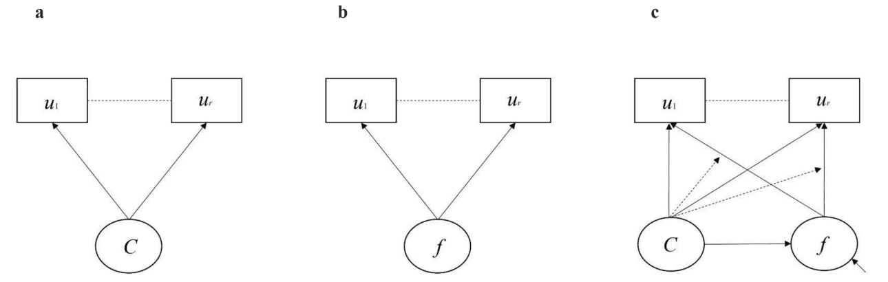
Model diagrams of a) latent class analysis; b) factor analysis; and c) factor mixture modelling. Adapted from Clark et al. (Clark et al., 2013). Note. Boxes represent observed categorical variables. u1 - ur = item responses on a questionnaire (e.g., SSAGA). Circles represent unobserved (i.e., latent variables). C = latent unordered class variable with k discrete classes. f = continuous factor / latent variable. Straight single-headed arrows indicate causal paths. Dashed straight lines indicate conditional independence of item responses after being explained by the latent variables C and/or f. Small diagonal arrow pointing to the factor in 1c is the factor variance.
In factor analysis, the pattern of observed responses is explained by a continuous latent variable called a factor (f) (see Fig. 1b). Observed responses are assumed to be conditionally independent once their covariance is explained by the common factor (see Clark et al., 2013 for details). For individual participants, each observed variable is decomposed into a combination of elements, including an intercept, a factor loading determining the influence of a factor on the measured variable, and the unique variance/error of the measured variable that is not explained by the factor loading (Bollen & Noble, 2011). The factor loadings capture the shared variance across the items explained by the factor. Participants are not assumed to be comprised of two or more subpopulations, but rather differences in pattern responses are determined by differences on the underlying factor. Thus, participants can be rank-ordered along a continuous dimension of the factor, which can be expressed through the derivation of observed variables called factor score estimates (Grice, 2001). Factor score estimates are an approximation of the sample distribution of the factor and express where each individual is located on the factor relative to the rest of the sample (Clark et al., 2013). However, a limitation of factor analysis is that participants in a sample are assumed to be from the same subpopulation with no qualitative or quantitative differences in the structure of the factor on which they are rank ordered.
FMM is a hybrid approach that combines the features of LCA and factor analysis (see Fig. 1c). The pattern of observed variables (i.e., item responses) is determined both by one or more latent classes and one or more factors (as indicated by the solid single-headed straight arrows) (see Clark et al., 2013 for details). Moreover, the factor means and variances (as indicated by the solid straight-headed arrow pointing from C to f) and factor loadings (as indicated by the dashed single-headed arrows) are allowed to vary as a function of class membership, which adds a great deal of flexibility to the model. FMM allows for the characterization of heterogeneity with latent classes by modeling the continuous factor and allowing the derivation of factor score estimates to quantify individual differences in scores within each class.
There are four variations of the FMM, ordered from the most restrictive to the least restrictive (i.e., the most to the least model parameters fixed to equality across classes) (see Fig. 2a – 2d). In the most restrictive model, the FMM-1, factor variances, observed variable thresholds (i.e., for categorical variables) or intercepts (i.e., for continuous variables), as well as factor loadings are fixed to equality across classes. This model suggests only differences in factor means across classes as would be expected for a non-normally distributed latent variable. For the FMM-2, factor variances are free to vary across classes, such that the factors are measured equivalently along the same continuum (i.e., factor means can be compared), but have different distributions. For the FMM-3, observed variable thresholds or intercepts vary across classes, suggesting differences in observed variables independent of differences in the factor (e.g., systematic response biases on questionnaire items within classes/groups), such that factor means can no longer be meaningfully compared across classes. Finally, for FMM-4, factor variances, thresholds/intercepts and factor loadings all vary across classes, such that the factors are no longer measured equivalently and do not have the same substantive interpretation across classes (e.g., items in a questionnaire are differentially related to the factor) (see Clark et al., 2013 for details).
Fig. 2.
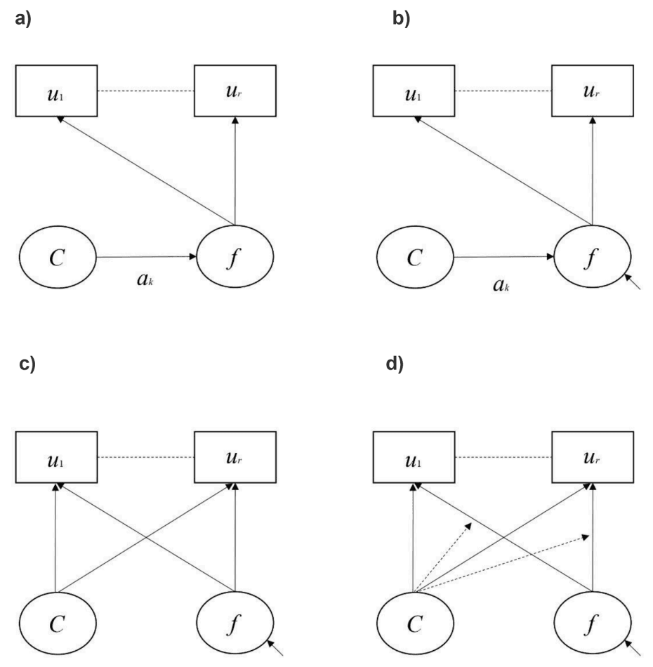
Model diagrams of different types of factor mixture models: a) FMM-1 – class membership determines differences in factor means (ak) only; b) FMM-2 – class membership determines differences in factor means and factor variances (as indicated by small single-headed diagonal arrow pointing to f; and c) FMM-3 – class membership determines observed variable thresholds/intercepts and the factor variance–covariance matrix is also free to vary across classes); FMM-4 – class membership determines factor loadings, observed variable thresholds/intercepts and the factor variance–covariance matrix is also free to vary across classes) Adapted from Clark et al. (Clark et al., 2013). Note. Boxes represent observed categorical variables. u1 - ur = item responses on a questionnaire (e.g., SSAGA). Circles represent unobserved (i.e., latent variables). C = latent unordered class variable with k discrete classes. f = continuous factor / latent variable. Straight single-headed arrows indicate causal paths. Dashed straight lines indicate conditional independence of item responses after being explained by the latent variables C and/or f.
We conducted the analyses following the procedure outline by Clark et al. (Clark et al., 2013) and using the Mplus program version 8.3 (L. K. Muthén, 2017). First, we fit factor analysis and latent class models to the SSAGA data for later comparison and to determine the upper bound for the number of factors and classes for the factor mixture models (Clark et al., 2013). For factor analysis, we used exploratory structural equation modelling (ESEM) and the weighted least square mean- and variance adjusted (WLSMV) estimator, which is the preferred estimator with ordered categorical (i.e., ordinal) data (Byrne et al., 2012; B. Muthén et al., 1997; L. Muthén & Muthén, 2017). ESEM is a hybrid of exploratory and confirmatory factor analysis, which takes an exploratory approach to modelling whilst also enabling model-data consistency to be evaluated with fit statistics (Asparouhov and Muthén, 2009, Marsh et al., 2014). We used a competing models strategy to determine whether the most parsimonious unidimensional model provided a superior fit compared to models with two or more factors (Hair et al., 2014a, Jöreskog, 1993). As it was possible that local dependencies between subsets of items could cause poor fit for a unifactorial model, we considered freely estimating correlated residuals (θδ) where consistent with theory and if significant after correction for Type I error using the Benjamini-Hochberg procedure (Benjamini and Hochberg, 1995, Silvia and MacCallum, 1988). To evaluate model-data consistency, we used a combination of absolute and approximate global fit statistics, as well as indices of local fit. We referred to the chi square (χ2) test statistic first, where p >.05 suggests the exact fit hypothesis for model-data consistency cannot be rejected (Hayduk et al., 2007, Marsh et al., 2004). We also report three approximate fit indices, the comparative fit index (CFI), the root mean square error of approximation (RMSEA), and the standardized root mean square residual (SRMR). Higher values for the CFI, and lower values of the RMSEA and associated 90% confidence interval (90 %CI), and SRMR are indicative of better fitting models. (Barrett, 2007, Byrne, 2013, Hair et al., 2014, Hayduk et al., 2007). To evaluate local fit, we used the matrix of correlation residuals (ε), which reveal discrepancies in the model estimated and observed bivariate correlations; where a pattern of ε greater than 0.10 indicates potential sources of poor local fit (Kline, 2015).
For latent class analysis (LCA), we used the maximum likelihood estimator with a chi square statistic and standard errors robust to non-normality (MLR) to handle the ordinal data. To determine the optimal number of classes in LCA, we followed the procedure outlined by Nylund et al. and Asparouhov and Muthen (Asparouhov and Muthén, 2009, Nylund et al., 2007). We generated 1–5-class models examining the inflection points for the trend in the log likelihood and Bayesian information criterion (BIC) values to identify a smaller range of plausible models (Nylund et al., 2007). From this smaller range of candidate models, the best log likelihood values were obtained for each number of classes tested using an initial number of random starting value perturbations and final stage optimizations (160, 32). The model was then rerun with double the number of random starting value perturbations and final stage optimizations (320, 64) to ensure that the analyses did not converge on local maxima in estimating the best log likelihood value (Asparouhov & Muthén, 2012; L. Muthén & Muthén, 2017).
Once the best log likelihood was replicated, each model was rerun to obtain the Lo–Mendell–Rubin (LMR) adjusted Likelihood Ratio Test (LRT) and Bootstrapped Likelihood Ratio Test (BLRT) by using the seed that resulted in the best log likelihood value specified as the starting value instead of random starts. Class enumeration was evaluated using a combination of fit statistics, including the entropy (E), BIC (Hair et al., 2014, Schwarz, 1978), the LMR adjusted LRT, and BLRT (Lo et al., 2001). Entropy is ranked from 0.00 to 1.00, with higher values indicating better class separation (Clark & Muthén, 2009). Lower BIC values indicate a better-fitting and more parsimonious model (Clark & Muthén, 2009). A non-significant p value for the LMR adjusted LRT and BLRT indicates that the k – 1 class model provides a better fit to the data than the k model or any subsequent k + 1 models (Nylund et al., 2007). The combination of these statistics has been determined to provide a relatively sensitive measure of the true number of classes (Nylund et al., 2007). Comparative model performance was also evaluated using the Bayesian conditional posterior probability, which quantifies the relative probability (p =.00–1.0) of model i compared to k models by dividing the exponentiated -12BIC for model i by the sum of the exponentiated -12BIC for k models:PrBIC(𝐻𝑖|𝐷)=exp[−12BIC(𝐻𝑖)]∑𝑘−1𝑗=0exp[−12BIC(𝐻𝑗)](Wagenmakers, 2007).
After determining the optimal number of classes, we then proceeded to test factor mixture models (FMM), using the MLR estimator to handle the ordinal data (L. Muthén & Muthén, 2017). We began with one-factor one-class and one-factor two-class models (Clark et al., 2013) and the most restrictive and parsimonious factor mixture model (i.e., FMM-1, different latent means only) before progressively relaxing equality constraints on the factor variance–covariance matrix (i.e., FMM-2); the item thresholds (i.e., FMM-3), and the factor loadings (i.e., FMM-4) to determine the best fitting model as indicated by the log likelihoods, entropy, BIC, and PrBIC(𝐻𝑖|𝐷)(Clark et al., 2013).We then systematically increased the number of specified classes for the one-factor model until reaching the k number of classes for the besting fitting LCA model. Finally, we compared the best-fitting factor mixture model to the best factor model and best latent class model using the BIC to determine the optimal representation of the data (Clark et al., 2013).
2.3. Delay discounting
In the Human Connectome Project (HCP), delay discounting was calculated for each individual using an extra-scanner Area Under Curve (AUC) approach, a model-free method that describes the delay discounting tendency of an individual (Green and Myerson, 2004, Myerson et al., 2001). Delays to reward-obtainment are fixed, but reward amounts are adjusted on a trial-by-trial basis based on a participant’s previous choice until an indifference point is reached. This represents the delay margin when the participant is more likely to choose a smaller but more immediate reward over a larger but delayed one, the theoretical indifference between the delayed reward and the estimated present subjective value of said reward to produce a discount curve using methods such as the AUC (Borges et al., 2016, Hamilton et al., 2015). The AUC for each participant is the total area of all trapezoids in his/her discounting curve (Frost & McNaughton, 2017). For more information, please see the Supplementary Methods.
2.4. Correlation between value-based decision-making network functional connectivity and substance use
Minimally preprocessed functional MRI data from the Human Connectome Project (HCP, Smith et al., 2013) was sourced for healthy adults of both genders (age range = 22–30). Only subjects with all four repeated resting-state fMRI sessions (first and second scan sessions with left–right and right-left phase encoding directions), who also possessed complete delay discounting, cognition, socioeconomic scores (i.e., education, income, and employment status) and mental health (i.e., depression, anxiety and somatic) measures, were included (n = 650). For a full account of the HCP neuroimaging acquisition and pre-preprocessing parameters, please see the Supplementary Methods.
The VS, ECS and PS brain masks were delineated using binary masks that combined regions of interest (ROIs) from both the Desikan-Killiany (Desikan et al., 2006) and Destrieux (Destrieux et al., 2010) parcellations (Table S1 in the Supplementary Methods and Results). All anatomical labels were extracted and merged using the FMRIB Software Library (Smith et al., 2004, https://fsl.fmrib.ox.ac.uk/fsl/). Resting-state functional connectivity scans in the HCP are divided into 4 subsets of scans, REST1 left–right (L-R), REST 1 R-L (REST1 R-L), REST2 L-R, REST2 R-L. For each subset, the resting state functional magnetic resonance imaging (rsfMRI) signal was averaged over all voxels comprising each ROI (node). The Pearson correlation coefficients between the regionally averaged signals for all nodes were then computed for each subset of scans per participant (i.e., each participants’ REST1 L-R scans forming one subset of n-by-n matrices, each participants’ REST1 R-L scans forming one subset of n-by-n matrices, and so on). To identify functional circuits within the VS, ECS and PS associated with Substance Use factor score estimates using the Network-Based Statistic (Zalesky et al., 2010), design matrices comprised of age (in years), sex, framewise displacement, transformed rates of discounting, cognitive scores, socioeconomic measures (i.e. employment, education and income), DSM-IV diagnosis of mental health conditions (i.e., depression, anxiety and somatic symptom disorder) and Substance Use factor score estimates as well as their standard errors, were correlated with the connectivity matrices of the VS, ECS and PS. Standard errors of the factor score estimates were included because measurement precision of the substance use factor was not uniform across the latent trait continuum due to the unipolar nature of the substance use construct (i.e., SSAGA items provide measurement of the presence of substance use problems, but there are no items that provide measurement of the low end of the continuum, see Figure S1). The measurement error is proportional to the distributional properties of the signal (i.e., a ‘multiplicative error-in-variable model’). However, this relationship is not monotonic. Thus, including the standard errors adjusts for this non-uniform measurement precision across the latent trait continuum. A composite subnetwork featuring edges that were common across all four subsets brain scans was compiled and visualized using BrainNet Viewer. This approach may help avoid issues of variability between visits (i.e. between REST1 and REST2) and hemispheric lateralization (Cao et al., 2021, Korponay and Koenigs, 2021, Ocklenburg and Mundorf, 2022). A family-wise error (FWE)-corrected p-value was calculated to identify the largest interconnected cluster of brain regions (5000 permutations) at a threshold of t = 2.5, p <.01. This threshold was selected from a range of possible values (1.0 to 5.0), the suitability of each was tested iteratively in increments of 0.5. Anything higher (i.e., greater than 3.0) resulted in nearly all edges no longer having a measure of association higher than the pre-set threshold. Put another way, thresholds above 2.5 would remove nearly all connections, leaving a subnetwork so sparse as to have almost no connections between brain regions. Pairwise connections were then visualized with BrainNet Viewer (Xia et al., 2013).
3. Results
3.1. Modelling of substance use behaviour
We found that a one-factor model, with two freely estimate error covariances (marijuana use with tobacco use θδ = 0.306, SE = 0.050 [95 %CI = 0.209, 0.403], p <.001 & hallucinogens θδ = 0.489, SE = 0.065 [95 %CI = 0.361, 0.617], p <.001) provided the best and most parsimonious representation of the latent structure of the data using ESEM (χ2 (18) = 26.069, p =.098, RMSEA = 0.019 [90 %CI = 0.000, 0.035], CFI = 0.998, SRMR = 0.025; see Fig. 3). Frequency of use for all substance classes loaded onto the common ‘Substance Use’ factor at p <.001 and there was only one correlation residual > 0.10 suggesting that the association been alcohol and tobacco had been slightly underestimated (see Table 1). In contrast, the competing two, three-, or four-factor models were all misspecified resulting in error warnings and indicating that they did not capture the data well. The results of the LCA suggested that a three-class model provided the best fit compared to one-, two-, or four-class models (see Table 2) whereas a five-class model was misspecified. The results of the LCA provide an upper bound for the number of classes that can be expected to fit the data for the FMM. This is because the LCA does not take account of the dimensional structure of the data and thus overestimates the number of classes (i.e., it takes more classes to fit the data than are needed because the factor structure of the variables is ignored). Thus, the three-class model represented the upper bound of the number of classes for the FMM.
Fig. 3.
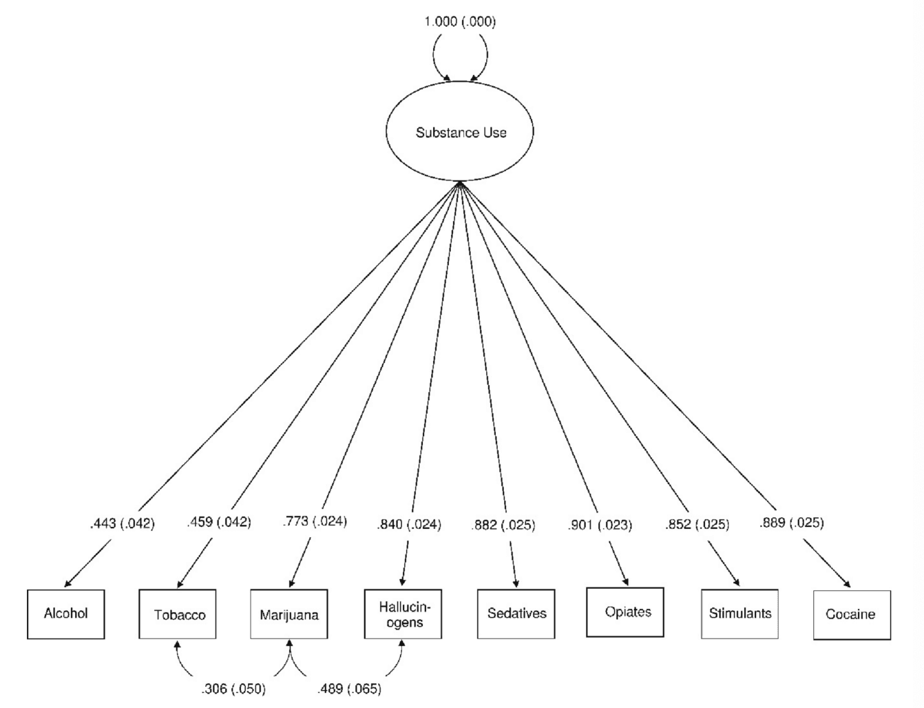
One-factor model of substance use in the Human Connectome Project participants. χ2(18) = 26.069, p =.098, RMSEA = 0.019 [90 %CI = 0.000, 0.035], CFI = 0.998, SRMR = 0.025. All factor loadings, as well as the two residual correlations, were statistically significant p <.001 N = 1,200.
Table 1. Correlation Residuals for the Two-Factor Model of Self-Reported Compulsivity as Modeled with the WLSMV Estimator.
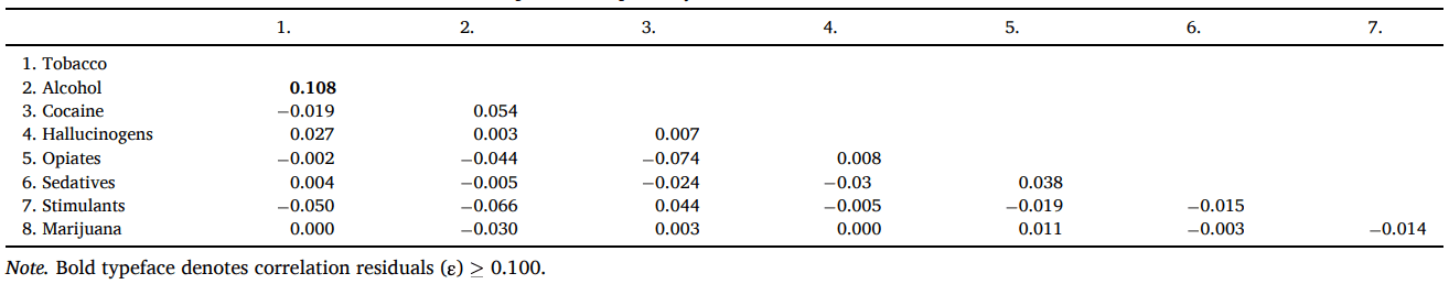
Note. Bold typeface denotes correlation residuals (ε) ≥ 0.100.
Table 2. Results of Exploratory Latent Class Analysis of Substance Use in Human Connectome Participants.
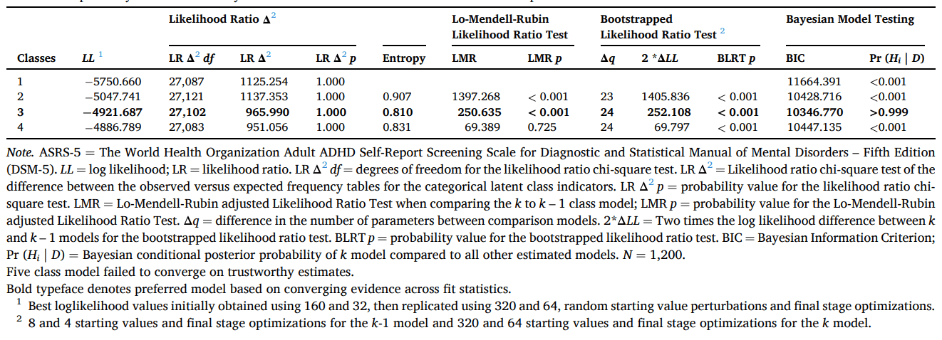
Note. ASRS-5 = The World Health Organization Adult ADHD Self-Report Screening Scale for Diagnostic and Statistical Manual of Mental Disorders – Fifth Edition (DSM-5). LL = log likelihood; LR = likelihood ratio. LR Δ2df = degrees of freedom for the likelihood ratio chi-square test. LR Δ2 = Likelihood ratio chi-square test of the difference between the observed versus expected frequency tables for the categorical latent class indicators. LR Δ2p = probability value for the likelihood ratio chi-square test. LMR = Lo-Mendell-Rubin adjusted Likelihood Ratio Test when comparing the k to k – 1 class model; LMR p = probability value for the Lo-Mendell-Rubin adjusted Likelihood Ratio Test. Δq = difference in the number of parameters between comparison models. 2*ΔLL = Two times the log likelihood difference between k and k – 1 models for the bootstrapped likelihood ratio test. BLRT p = probability value for the bootstrapped likelihood ratio test. BIC = Bayesian Information Criterion; Pr (Hi | D) = Bayesian conditional posterior probability of k model compared to all other estimated models. N = 1,200.
Five class model failed to converge on trustworthy estimates.
Bold typeface denotes preferred model based on converging evidence across fit statistics.
1Best loglikelihood values initially obtained using 160 and 32, then replicated using 320 and 64, random starting value perturbations and final stage optimizations.
28 and 4 starting values and final stage optimizations for the k-1 model and 320 and 64 starting values and final stage optimizations for the k model.
We then estimated FMMs (FMM-1 to FMM-4) with the unidimensional Substance Use factor and one- to three-class models (see Table 1). We also estimated these models specifying a zero-inflated class with factor loadings and factor variances fixed at zero, and factor means freely estimated and the starting values of the item thresholds set to low probability of endorsement. Finally, we estimated two- and three-class non-parametric FMMs with factor variances fixed at zero. These models are indicated when the distributions of the factor are non-normal, such as the zero-inflated distribution of clinical variables in non-clinical populations, including substance use in the current sample. Most of these models failed to converge on trustworthy estimates, indicating misspecified (i.e., ill-fitting) models. A two-class model with class varying factor variances and thresholds (FMM-3) provided a reasonable fit to the data, although class separation was relatively poor (LL = -4,328.817, E = 0.707, BIC = 10168.916). However, the one-class one-factor model provided a superior fit to the data (LL = 4,901.545, BIC = 10086.602) as revealed by the Bayes factor, which provided very strong evidence in favour of this model compared to the two-class FMM-3 (BF01 = 7.486140810132e+17).
The latent variable distribution plot is provided in Fig 4 and indicates some zero-inflation in the distribution. We generated factor score estimates using the regression method (Grice, 2001, Muthén and Muthén, n.d..) for each participant based on the one-class, one-factor solution for subsequent analysis with the neuroimaging data. The information function for the Substance Use latent variable is shown in Figure S2. Information (I) can be converted into a standard metric of reliability (rxx) using the formula [𝑟𝑥𝑥=1−(1/𝐼)]and is plotted in standardized units along the latent trait continuum (i.e., M = 0, SD = 1) (Toland, 2014). Not surprisingly, measurement precision was highest above the mean where it was approximately rxx = 0.6, peaking at + 2SD (rxx = 0.93), before dropping below rxx = 0.6 again at ∼+3.5SD. This was due to the unipolar nature of the construct ‘Substance Use’ (i.e., there is no item content to measure the adaptive end of the continuum (Lucke, 2015) beyond low substance use).
Fig. 4.
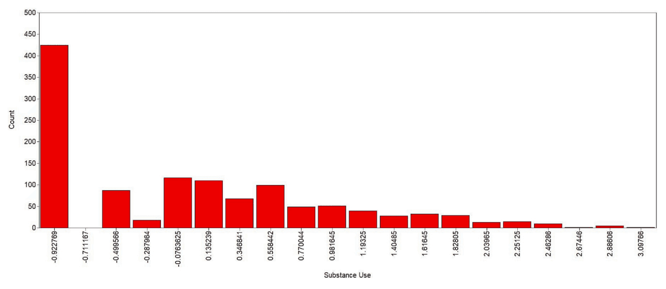
Latent variance distribution plot for the ‘Substance Use’ factor. N = 1,200. The × axis is defined in standardized units, with a mean of zero and standard deviation of one. The metric of the y axis is the number of participants in the sample with that value of the latent variable.
We also regressed the Substance Use factor onto sex, age, maternal and paternal substance use history to determine if these demographic variables explained variance in the substance use behaviour of participants (see Figure S2). We found that males (γ = -0.249, SE = 0.033, p <.001) and older participants (γ = 0.065, SE = 0.033, p =.051) tended to have higher substance use, as did those participants whose mother (γ = 0.097, SE = 0.032, p =.002) and father (γ = 0.103, SE = 0.031, p =.001) had a substance use history. However, the effect sizes were very small (R2 ≤ 0.011), except for sex (R2 = 0.062). The brant Wald test for proportional odds was only significant for sex and marijuana use (χ2(4) = 15.173, p =.004), indicating that the pattern of endorsement of frequency of use was different between males and females.
Note. Model figure is displayed using symbols from the McArdle-McDonald reticular action model (RAM) (McArdle, 1980). Observed (also measured or manifest) variables are represented as rectangles. The factor (latent variable or construct) is represented as a large ellipse. The double-headed, curved arrow pointing to the factor is the latent variable variance. Straight, single-headed arrows from the large ellipse to observed variables reflect factor loadings. Curved, double-headed arrows between rectangles are error covariances/residual correlations.
3.2. Network-based Statistic modelling
Significant subnetworks were observed when functional connectivity of regions recruited by the VS, ECS and PS as well as the insula, caudate, putamen and intraparietal sulcus were correlated with the design matrix. All subnetworks were negatively correlated with delay discounting, cognitive scores, employment, education and income status but positively correlated with DSM-IV diagnoses of depression, anxiety and somatic problems, as well as substance use factor score estimates and their standard errors. Given that this NBS analyses was performed independently on each subset of brain scans (i.e. REST1 L-R, REST1 R-L and so on), four separate significant subnetworks were obtained. A composite list was then compiled consisting entirely of connections found across all four subsets. This composite list of connections is represented graphically in Fig. 5.
Fig. 5.
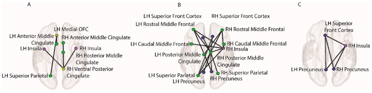
Composite connections found in each of the four significant (p < 0.05) subnetworks identified by the NBS from subsets of HCP resting state brain scans (i.e., REST 1 L-R, REST1 R-L, REST2 L-R, REST2 R-L). All subnetworks were negatively correlated with delay discounting, cognitive scores, employment, education, and income status but positively correlated with DSM-IV diagnoses of depression, anxiety, and somatic problems as well as substance use factor score estimates and their standard errors. (A) Functional connections within the ECS are positively correlated with Substance Use factor score estimates; (B) VS functional connections with regions of the ECS and PS were positively correlated with Substance Use factor score estimates; (C) ECS functional connections with regions of the PS were positively correlated with Substance Use factor score estimates.
Connections involving regions of the VS were left medial OFC to the left superior parietal and left anterior middle cingulate as well as the right ventral posterior cingulate to the right anterior middle cingulate, right posterior middle cingulate and bilateral insula. Connections involving regions of the ECS were the bilateral superior parietal cortex to the right posterior middle cingulate, the bilateral rostral middle cingulate to the right posterior middle cingulate, the right posterior middle cingulate to the bilateral precuneus, left rostral middle frontal to right precuneus, left superior parietal and right posterior middle cingulate to the bilateral superior frontal cortex, left superior parietal, right posterior middle cingulate, bilateral rostral middle frontal and bilateral caudal middle frontal to the right insula and right rostral middle frontal to left posterior middle cingulate. Connections involving regions of the PS were the bilateral precuneus to the left superior frontal cortex and right insula, as well as the left superior frontal cortex to the right insula.
4. Discussion
The aim of our study was to identify neuroimaging susceptibility biomarkers of SUDs in young adults from the Human Connectome Project (HCP). Rather than being taxonomic in structure, the continuity hypothesis suggests that there is a continuum of substance use extending from normal to problematic use in the population (Borsboom et al., 2016). This continuity has previously been demonstrated for alcohol use (Krueger et al., 2004). However, it also possible that latent classes are embedded within the continuum of substance use problems suggesting that hybrid models that combine dimensional and categorical measurement may better fit the data (B. Muthén, 2006). Here we used factor mixture modelling, a hybrid modelling approach that combines factor analysis and latent class analysis, which is well-suited to characterizing the latent structure of psychiatric phenomena, such as substance use behaviour (Clark et al., 2013, Miettunen et al., 2016). We hypothesized that a single continuum of substance use frequency and severity with a distinct zero-inflated latent class would best characterize the substance use behaviour in our sample of young adults from the HCP.
Our hypothesis of a single substance use continuum that combined frequency of use across all substance classes was supported. Each of the substances loaded moderately (alcohol and tobacco) to strongly (marijuana, hallucinogens, sedatives, opiates, stimulants, cocaine) on a unidimensional factor, suggesting that a single continuum adequately captures and describes covariation of substance use across all classes within the sample. In contrast, hybrid models with two or more latent classes, including a zero-inflated class characterizing a proportion of individuals with low frequency of use across all substance classes, failed to provide a good fit to the data. Thus, despite evidence of some zero-inflation in the continuum of substance use behaviour, a hybrid model with a distinct class of individuals with low scores did not provide a good fit to the data as compared to a model with a single continuous dimension. These findings indicated that young adults from the HCP could be rank-ordered along a single continuum of substance use frequency and severity. Furthermore, findings indicated that factor score estimates generated from this continuum could be analyzed with functional connectivity data to examine brain-behaviour associations and identify the functional neural substrates of substance use behaviour. Such dimensional analyses are better situated to detect meaningful brain-behaviour associations compared to categorical distinctions and speak to the utility of a dimensional enhancement approach to researching SUDs (Cuthbert, 2014).
4.1. Functional connectivity within and between the VS, ECS, and PS is associated with substance use behaviour
We found that connections between the VS, ECS and PS were positively correlated with substance use factor score estimates, as well as incidence of depression, anxiety, and somatic problems, but was negatively correlated with delay discounting (i.e., choice impulsivity). These findings agree with our previously stated hypotheses and can be interpreted in the context of reward-based valuation and decision making (i.e., sensation seeking), which represents a predisposing factor for SUDs (Verdejo-Garcia & Albein-Urios, 2021). Sensation-seeking utilizes a goal-directed approach system (J. A. Gray, 1990) geared towards satisfying the need for rewarding experiences (Zuckerman, 1994). This behaviour is a part of the impulsivity construct (Miranda-Olivos et al., 2022) and may motivate substance use (including poly-substance use) (Chakroun et al., 2004, Woicik et al., 2009). Regions of the ECS (and PS) could provide goal-directed value signals to the medial OFC (VS), aiding decision-making in pursuit of addictive substances. Even among non-dependent drug users, functional activation (Filbey & Dunlop, 2014) and connectivity have been reported previously (Ersche et al., 2020). Both studies highlight the impact of regions such as the precuneus, superior frontal cortex (both PS), posterior parietal and lateral prefrontal cortex (ECS) in preventing a non-dependent drug user from becoming dependent. Connections between the VS and PS may contribute to the development of interoceptive thoughts revolving around the pleasurable sensations experienced during drug use, but the numerous connections with ECS regions could help to restrict the impact of these thoughts and the potential transition to dependence.
It has been theorized that a delicate balance may exist between valuation- and control-based regions of the brain that regulate impulsive behaviours, and that disruption of this balance may underpin the development of addictive behaviours (Xie et al., 2014; T. Zhai et al., 2015). More recent studies indicate that regions of the ECS (the lateral prefrontal cortex in the context of the current study) and PS (the superior frontal cortex, once again in the context of this study) are implicated in top-down inhibitory control (Ersche et al., 2020). Here, we observed a positive correlation between substance use factor score estimates and connections between regions of the VS, ECS and PS among poly-drug users. We thus infer that although these participants may favour mixing-and-matching various substances to heighten their consumptive experiences (connections between the VS and ECS, PS), they may not have developed full-on dependency owing to the protective effects of connections within and between the ECS (particularly the lateral prefrontal cortex) and PS (particularly the superior frontal cortex). The potential role of both the lateral prefrontal and superior frontal cortices in potentially staving off dependency may be further emphasised via the concomitant negative correlation between participants’ delay discounting scores and network connectivity. The more impulsive one becomes, the stronger the connections within and between the ECS and PS, a possible countermeasure to preserve the balance between the value of poly-drug use and top-down cognitive control.
The lateral prefrontal, posterior cingulate and posterior parietal cortices emerged as hubs within the ECS (Fig. 5). The lateral prefrontal cortex orients attention and subserves approach behaviour towards rewards, disregarding the consequences of risky behaviour during sensation-seeking (Cservenka et al., 2013, Davidson et al., 2004). Left lateral prefrontal cortex activation is associated with both impulsivity and sensation-seeking (Chase et al., 2017) by encoding stimulus-outcome associations (Boorman et al., 2016), preparatory attention (van Schouwenburg et al., 2010, Wallis et al., 2015, Woolgar et al., 2015), optimistic bias (Garrett et al., 2014), and free-choice (Cho et al., 2016). The posterior parietal cortex is associated with decision-making and is a reliable predictor of risk-taking (Gilaie-Dotan et al., 2014) and risk preference (Teti Mayer et al., 2021), while the posterior cingulate cortex is thought to encode the neuroeconomic value of the subject (in this case, the drug of choice) (Brosch et al., 2013). Connections from the posterior parietal cortex extend to the medial orbitofrontal cortex and superior frontal cortex, while the right posterior middle cingulate is connected to the superior frontal cortex and precuneus (Fig. 5B). These findings suggest that impulsive sensation-seekers willingly engage in goal-directed poly-drug use (risky behaviour), with the optimistic view that they will once again experience the same pleasurable sensations as before by consuming their preferred substance(s).
Interestingly, connections were observed between the insula and regions of the VS, ECS and PS. The insula is believed to be involved in attention orientation towards rewards (Anderson et al., 2016, Farrant and Uddin, 2015), being sensitive towards cues signalling preferred rewards (Goudriaan et al., 2010, Kober et al., 2016, Limbrick-Oldfield et al., 2013). Increased functional connectivity was observed between the insula and the ventral cingulate cortex (VS), as well as regions of the ECS (i.e., bilateral rostral and caudal middle frontal cortex, bilateral posterior middle cingulate cortex and left superior parietal cortex), as well as the PS (i.e., bilateral precuneus and left superior frontal cortex). These results suggest that drug users may have a fixation towards thoughts of drugs as the reward of choice (VS - posterior cingulate cortex), fuelled in part by memories of previous use and those outcomes (PS). This increased connectivity was negatively correlated with delay discounting scores (i.e., steeper discounting or a preference for risker choices), particularly reflected by connections between the insula and the prefrontal cortex. These results further suggests the influence of reward-related attentional bias on value-based decision-making, possibly making it more challenging to accept delayed rewards in the face of faster returns (Clewett et al., 2014). Nevertheless, connections involving ECS regions may balance poly-substance pursuit (and the perceived benefits of its consumption), thereby stalling or even preventing dependence.
Our findings can be interpreted from two perspectives. First, the relationship between delay discounting and functional connectivity among substance users. As mentioned earlier, Owens et al. (2019) performed a systematic review of the literature surrounding functional and structural connectivity among substance users and its relationship with delay discounting. Our results concur with some of the studies highlighted by Owens et al. For example, Camchong et al. (2011) reported increased connectivity between the anterior cingulate cortex and the dorsolateral prefrontal cortex among cocaine dependents. Clewett et al. (2014) also reported similar findings among smokers, involving the dorsolateral prefrontal and posterior parietal cortices correlated (Clewett et al., 2014). Contreras-Rodriguez et al. (2015) observed increased connectivity between the ventral striatum (site of the nucleus accumbens) and the anterior cingulate cortex. All three studies showed positive correlation with delay discounting, in contrast to our findings. While regions like the dorsolateral prefrontal and posterior parietal cortices appear to act as hubs in our study, we utilized data for use patterns across eight different substances. As observed by Morris et al (2022) the presence of multiple substances, combined with increased use severity can cause changes in connectivity correlates. It may also reflect the increased value attributed to taking combinations of substances as a means of achieving pleasure or pain relief. Individuals may crave for their drug(s) of choice, and may be willing to accept smaller doses if it can be procured more quickly (Loganathan & Ho, 2021). They may also view mixing-and-matching addictive substances as a quick and easy way to reach their desired state, instead of utilizing non-substance related means.
The second perspective revolves around utilization of our findings. Research indicates that while most studies focus on chronic, severe substance abuse (i.e. addiction), a majority of the population experiences mild-to-moderate symptoms of substance use disorder and account for more substance-use harms compared to those with severe SUDs (Asken et al., 2007, McLellan et al., 2022). Recently, McLellan et al (2022) shone the spotlight on ‘preaddiction’, a term describing the state of mild-to-moderate substance use disorders that could pre-date addiction. They also highlight a lack of objective assessments to detect individuals in a preaddiction state (McLellan et al., 2022). We would like to propose the continuum reported here, along with the functional hubs and edges correlated with both factor score estimates of substance use behaviour and delay discounting scores, as a possible neurobiological assessment to be used with individuals in the preaddiction state. We further propose that our models be used in tandem with existing diagnostic criteria as contained within the DSM-5 (Asken et al., 2007) when assessing patients with substance use disorder.
The results of our study are tempered by methodological limitations. First, it is possible for mixture and hybrid modelling to yield solutions that are idiosyncratic to specific samples (Borsboom et al., 2016). Thus, it will be important to replicate the findings of a continuous, unidimensional spectrum of substance use frequency and severity in other samples and determine if the same neurobiological substrates are uncovered. Unfortunately, we did not have an independent sample with which to replicate our results. The one-factor, one-class solution we converged on may reflect the non-clinical characteristics of the sample, in which only a small subset of participants reported use of illicit psychoactive substances, including hallucinogens, cocaine, stimulants, and opiates. It is possible that a sample with more varied substance use profiles would yield a multiple class solution. Furthermore, the Semi-Structured Assessment for the Genetics of Alcoholism (SSAGA) does not measure frequency of use across all substance classes with the same level of granularity and precision (Bucholz et al., 1994). For example, alcohol dependency is measured using SSAGA Alcohol DSM4 Dependency Diagnosis with two categories (i.e., 1 for no, 5 for yes); tobacco dependency via the SSAGA FTND Score (Fagerstrom FTND test for nicotine dependence) with seven categories (0 – 3, not dependent; 4 – 6, dependent); lifetime use of cocaine, stimulants, opiates, and sedatives with three categories (i.e., 0, never used; 1, 3 – 5 occasions and 5, more than 6 occasions); lifetime use of hallucinogens with four categories (i.e. 0, never used; 1, 1 – 2 occasions, 2, 6–10 occasions and 5, more than 10 occasion); lifetime marijuana use with six categories (i.e., 0, never used; 1, 1 – 5 occasions; 2, 6 – 10 occasions; 3, 11 – 25 occasions; 3, 26 – 50 occasions; 3, 51 – 100 occasions; 4, 101 – 999 occasions; 5, more than 1000 occasions). This may have introduced constraints on the latent structure of the substance use continuum, as well as the number of latent classes that could be identified. It will be important in future studies to use a consistent scale for measuring frequency and severity of use across substance classes, as well as to replicate the findings in an independent sample for purposes of external validation. Measurement of substance use frequency; severity and its neurobiological correlates were cross-sectional rather than longitudinal. Thus, we are unable to determine whether the properties of network connectivity of the VS, PS, and ECS reflect an underlying vulnerability to substance use or are the consequences of substance use (Ersche et al., 2010). Future work could measure functional connectivity within and between these networks in youth and determine whether network properties predict individual differences in substance use behaviour longitudinally. Lastly, the period when the SSAGA Assessment was conducted in relation to brain scan collection could have introduced some variance in the relationship between substance use and functional connectivity, since use measures may be correlated with time of year (e.g., weekend, holiday season, etc.).
5. Conclusions
In summary, we provide evidence of susceptibility biomarkers that index a continuum of substance use frequency/severity that has implications for identification of those at risk for SUDS. Furthermore, functional connectivity of decision-making systems was positively correlated with substance use severity and negatively correlated with delay discounting. The orbitofrontal, dorsolateral prefrontal, and posterior parietal cortices emerged as hubs connecting other regions of the VS, ECS and PS, possibly signalling increased valuation of multiple substance as the reward of choice. These findings could be used in combination with other clinical findings to identify individuals currently in a preaddiction state and at risk of transitioning into addiction. Prospective longitudinal studies that predict transition to SUDs based on the functional connectivity profiles identified in this study as susceptibility biomarkers would be needed to confirm our findings.