Introduction

The Adolescent Brain Cognitive Development (ABCD) Study offers an unprecedented opportunity to comprehensively characterize the emergence of pivotal behaviors and predispositions in adolescence that serve as risk or mitigating factors in physical and mental health outcomes (Jernigan et al., 2018; Volkow et al., 2018). Data collection was launched in September 2016, with the primary objective of recruiting over 11,000 participants - including more than 800 twin pairs - across the United States over a two-year period. These 9–10-year-olds will be followed over a period of ten years. This age window encompasses a critical developmental period, during which exposure to substances and onset of many mental health disorders occur. The ABCD Study is the largest project of its kind to investigate brain development and peri-adolescent health, and includes multimodal brain imaging (Casey et al., 2018), bioassay data collection (Uban et al., 2018), and a comprehensive battery of behavioral (Luciana et al., 2018) and other assessments (Bagot et al., 2018; Barch et al., 2018; Lisdahl et al., 2018; Zucker et al., 2018). The longitudinal design of the study, large diverse sample (Garavan et al., 2018), and open data access policies will allow researchers to address many significant and unanswered questions.

Large Scale Multimodal Image Acquisition

The past few decades have seen increasing interest in the development and use of non-invasive in vivo imaging techniques to study the brain. Rapid progress in MRI methods has allowed researchers to acquire high-resolution anatomical and functional brain images in a reasonable amount of time, which is particularly appealing for pediatric and adolescent populations. The ABCD Study builds upon existing state-of-the-art imaging protocols from the Pediatric Imaging, Neurocognition Genetics (PING) study (Jernigan et al., 2016) and the Human Connectome Project (HCP) (Van Essen et al., 2012) for the collection of multimodal data: T₁-weighted (T₁w) and T₂-weighted (T₂w) structural MRI (sMRI), diffusion MRI (dMRI), and functional MRI (fMRI), including both resting-state fMRI (rs-fMRI) and task-fMRI (Casey et al., 2018). The fMRI behavioral tasks include a modified monetary incentive delay task (MID) (Knutson et al., 2000), stop signal task (SST) (Logan, 1994) and emotional n-back task (EN-back) (Cohen et al., 2016). These tasks were selected to probe reward processing, executive control, and working memory, respectively (Casey et al., 2018). The ABCD imaging protocol was designed to extend the benefits of high temporal and spatial resolution of HCP-style imaging (Glasser et al., 2016) to multiple scanner systems and vendors. Through close collaboration with three major MRI system manufacturers (Siemens, General Electric and Philips), the ABCD imaging protocol achieves HCP-style temporal and spatial resolution on all three manufacturers’ 3 Tesla systems (Siemens Prisma and Prisma Fit, GE MR 750, and Philips Achieva dStream and Ingenia) without the use of non-commercially available system upgrades.

To help address the challenges of MRI data acquisition with children, real-time motion correction and motion monitoring is used when available to maximize the amount of usable subject data. The prospective motion correction approach, first applied in PING, uses very brief “navigator” images embedded within the sMRI data acquisition, efficient image-based tracking of head position, and compensation for head motion (White et al., 2010). Significant reduction of motion-related image degradation is possible with this method (Brown et al., 2010; Kuperman et al., 2011; Tisdall et al., 2016). Prospective motion correction is currently included in the ABCD imaging protocol for the sMRI acquisitions (T1w and T2w) on Siemens (using navigator-enabled sequences (Tisdall et al., 2012)) and General Electric (GE; using prospective motion (PROMO) sequences (White et al., 2010)) and will soon be implemented on the Philips platform.

Real-time motion monitoring of fMRI acquisitions has been introduced at the Siemens sites using the Frame-wise Integrated Real-time Motion Monitoring (FIRMM) software (Dosenbach et al., 2017). This software assesses head motion in real-time and provides an estimate of the amount of data collected under pre-specified movement thresholds. Operators are provided a display that shows whether our movement criterion (>12.5 minutes of data with framewise displacement (FD (Power et al., 2014)) < 0.2 mm) has been achieved. FIRMM allows operators to provide feedback to participants or adjust scanning procedures (i.e., skip the final rs-fMRI run) based on whether the criterion has been reached. Future deployment of FIRMM for GE and Philips sites is planned.

Challenges of Multimodal Image Processing

A variety of challenges accompany efforts to process multimodal imaging data, particularly with large numbers of subjects, multiple sites, and multiple scanner manufacturers. Head motion is a significant issue, particularly with children, as it degrades image quality, and potentially biases derived measures for each modality (Fair et al., 2012; Power et al., 2012; Reuter et al., 2015; Satterthwaite et al., 2012; Van Dijk et al., 2012; Yendiki et al., 2013). Censoring of individual degraded frames and/or slices is one approach used in the literature to minimize contamination of dMRI and fMRI measures (Hagler et al., 2009; Power et al., 2014; Siegel et al., 2014). Correcting image distortions is important because anatomically accurate, undistorted images are essential for precise integration of dMRI and fMRI images with anatomical sMRI images. Furthermore, correcting distortions reduces variance in longitudinal change estimates caused by differences in the precise position of the subject in the scanner (Holland and Dale, 2011). Because the ABCD MRI acquisition protocol relies on high density, phased array head coils, image intensity inhomogeneity can be dramatic and can, if not properly corrected in sMRI images, lead to inaccurate brain segmentation or cortical surface reconstruction. As described in Methods, the ABCD image processing pipeline includes general and modality-specific corrections to addresses these known challenges of head motion, distortion, and intensity inhomogeneity. The image processing pipeline is expected to evolve over time to incorporate improvements and extensions in order to better address the challenges of large-scale multimodal image processing and analysis and to respond to future challenges specific to longitudinal analyses, such as the possibility of scanner and head coil upgrade or replacement during the period of study.

Data as a Public Resource

The advent of large-scale data sharing efforts and genomics consortia has created exciting opportunities for biomedical research. The availability of datasets drawn from large numbers of subjects enables researchers to address questions not feasible with smaller sample sizes. Public sharing of processing pipelines and tools, in addition to raw and processed data, facilitates replication studies, reproducibility, and meta-analyses with standardized methods, and encourages the application of cross-disciplinary expertise to develop new analytic methods and test new hypotheses. To this end, data and methods sharing is an integral component of the ongoing ABCD Study. Processed data and tabulated region of interest (ROI) based analysis results are made publicly available via the National Institute for Mental Health (NIMH) Data Archive (NDA). Processing pipelines themselves are shared as platform-independent data processing tools.

Aims and Scope

This manuscript is intended to serve as a reference for users of neuroimaging data from ABCD Data Release 2.0, made publicly available in March 2019 and amendment ABCD Fix Release 2.0.1, made publicly available in July 2019. Our focus is to provide a detailed overview of the image processing and analysis methods used to prepare imaging and imaging-derived data for public release. Other imaging-related aspects of the ABCD Study, including image acquisition, data curation, and data sharing are briefly described. Some preliminary characterizations of the baseline data are included in this report; more in-depth elaborations on baseline participant characterization, neuroimaging descriptive statistics, and quality control optimization are planned for separate reports. We anticipate that this material will be useful to ABCD collaborators and the broader scientific community for accelerating neuroimaging research into adolescent brain and cognitive development.

Methods

Overview

The ABCD Data Analysis and Informatics Center (DAIC) performs centralized processing and analysis of MRI data from each modality, leveraging validated methods used in other large-scale studies, including the Alzheimer’s Disease Neuroimaging Initiative (ADNI) (Mueller et al., 2005), Vietnam Era Twin Study of Aging (VETSA) (Kremen et al., 2010), and PING (Jernigan et al., 2016). We used a collection of processing steps contained within the Multi-Modal Processing Stream (MMPS), a software package developed and maintained in-house at the Center for Multimodal Imaging and Genetics (CMIG) at the University of California, San Diego (UCSD) that provides large-scale, standardized processing and analysis of multimodality neuroimaging data on Linux workstations and compute clusters. This toolbox contains primarily MATLAB functions, as well as python, sh, and csh scripts, and C++ compiled executables and relies upon a number of publicly available neuroimaging software packages, including FreeSurfer (Fischl, 2012), Analysis of Functional NeuroImages (AFNI) (Cox, 1996), and FMRIB Software Library (FSL) (Jenkinson et al., 2012; Smith et al., 2004). The processing pipeline described in this manuscript was used for the ABCD Data Release 2.0, available in March 2019, and a beta testing version has been made publicly available as a self-contained, platform-independent executable (https://www.nitrc.org/projects/abcd_study). Imaging statistics shown here include the amended ABCD Fix Release 2.0.1 data published in July 2019.

As described above, the ABCD image acquisition protocol includes sMRI, dMRI, and fMRI data. While there are many modality-specific details of the processing and analysis pipeline that will be discussed below, we conceptualize five general stages of processing and analysis.

1. Unpacking and conversion: DICOM files are sorted by series and classified into types based on metadata extracted from the DICOM headers, and then converted into compressed volume files with one or more frames (time points). DICOM files are also automatically checked for protocol compliance and confirmation that the expected number of files per series was received.

2. Processing: Images are corrected for distortions and head motion, and cross-modality registrations are performed (Fig. 1A).

3. Brain segmentation: The cortical surface is reconstructed and subcortical and white matter regions of the brain are segmented.

4. Analysis: We carry out modality-specific, single-subject level analyses and extract imaging-derived measures using a variety of regions of interest (ROIs).

5. Summarization: ROI analysis results are compiled across subjects and summarized in tabulated form. To provide context for how the centralized image processing is performed in preparation for the public release of data, we will also briefly describe MRI data acquisition, quality control, and data and methods sharing. A diagram documenting the various outputs of the processing pipeline can be found in Figure 1B.

Figure 1.

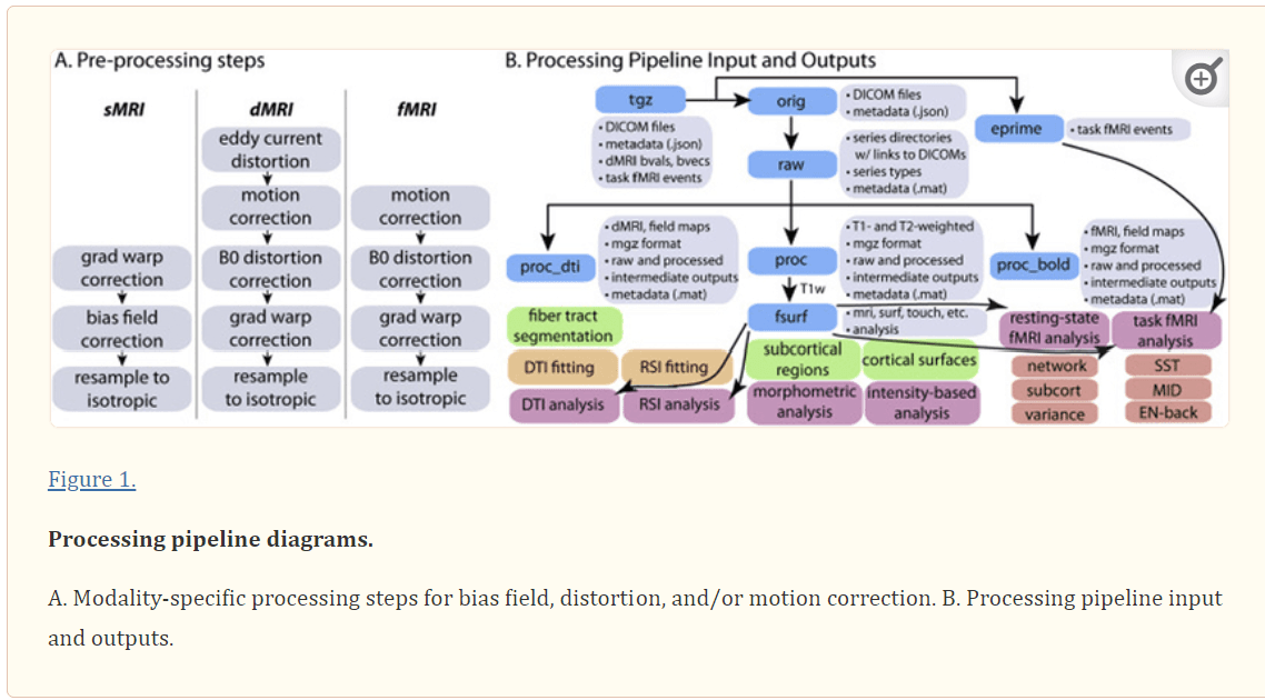
Processing pipeline diagrams. A. Modality-specific processing steps for bias field, distortion, and/or motion correction. B. Processing pipeline input and outputs.

Image Acquisition

A standard scan session includes sMRI series (T₁w and T₂w), one dMRI series, four rs-fMRI series, and two task-fMRI series for each of three tasks (MID, SST, and EN-back). Minimal details of the imaging protocol are provided here to contextualize the following description of the processing pipeline; additional details have been published previously (Casey et al., 2018). The scan order is fixed as follows: localizer, 3D T1-weighted images, 2 runs of resting state fMRI, diffusion weighted images, 3D T2-weighted images, 2 runs of resting state fMRI and then 3 fMRI tasks (MID, SST and EN-back). The fMRI tasks are randomized across subjects, except siblings receive the same order of tasks. Task order is held constant across longitudinal waves of the study for each subject (see Casey et al 2018). Scan sessions typically require ~2 hours to complete, including a mid-session rest break if the child requests one; they are sometimes split into two separate sessions that take place within one week of each other (3.5% of participants included in ABCD Data Release 2.0/Fix Release 2.0.1). Over 79% of the participants included in ABCD Data Release 2.0/2.0.1 successfully completed the entire image acquisition protocol. Some participants who are unable to complete one or more of the fMRI behavioral tasks (MID, SST, or EN-back), instead perform the missing task or tasks outside the scanner on a laptop computer1.

The T₁w acquisition (1 mm isotropic) is a 3D T₁w inversion prepared RF-spoiled gradient echo scan using prospective motion correction, when available (currently only on Siemens and GE scanners) (Tisdall et al., 2012; White et al., 2010). The T₂w acquisition (1 mm isotropic) is a 3D T₂w variable flip angle fast spin echo scan, also using prospective motion correction when available. Prospective motion correction has not been implemented for dMRI or fMRI acquisition. The dMRI acquisition (1.7 mm isotropic) uses multiband EPI (Moeller et al., 2010; Setsompop et al., 2012) with slice acceleration factor 3 and includes 96 diffusion directions, seven b=0 frames, and four b-values (6 directions with b=500 s/mm², 15 directions with b=1000 s/mm², 15 directions with b=2000 s/mm², and 60 directions with b=3000 s/mm²). The fMRI acquisitions (2.4 mm isotropic, TR=800 ms) also use multiband EPI with slice acceleration factor 6. Each of the dMRI and fMRI acquisition blocks include fieldmap scans for B₀ distortion correction. The imaging protocol was developed in collaboration with each scanner manufacturer using commercially available system upgrades, and where possible, product sequences. Imaging parameters were made as similar as possible across scanner manufacturers, although some hardware and software constraints were unavoidable (for details, see Appendix).

Unpacking and Conversion

After encrypted data is electronically sent from participating sites to the DAIC, data are automatically copied to a network attached, high capacity storage device (Synology, Taiwan) using a nightly scheduled rsync operation. The contents of this device are automatically inventoried using the metadata-containing JSON files to categorize series into the different types of imaging series: T₁w, T₂w, dMRI, rs-fMRI, MID-task-fMRI, SST-task-fMRI, and EN-back-task-fMRI. Missing data are identified by comparing the number of series received of each type to the number of series collected for a given subject, as entered into a REDCap database entry form by the site scan operators. The numbers of received and missing series of each type for each subject are added to the ABCD REDCap database. Using web-based REDCap reports, DAIC staff identify participants with missing data, and either request the data to be re-sent by acquisition sites or address technical problems preventing the data transfer. After receiving imaging data at the DAIC, the tgz files are extracted. For dMRI and fMRI exams collected on the GE platform prior to a software upgrade2, this step includes the offline reconstruction of multiband EPI data from raw k-space files into DICOM files, using software supplied by GE.

Protocol Compliance and Initial Quality Control

Using a combination of automated and manual methods, we review datasets for problems such as incorrect acquisition parameters, imaging artifacts, or corrupted data files. Automated protocol compliance checks providing information about the completeness of the imaging series and the adherence to the intended imaging parameters. Out-of-compliance series are reviewed by DAIC staff, and sites are contacted if corrective action is required. Protocol compliance criteria include whether key imaging parameters, such as voxel size or repetition time, match the expected values for a given scanner. For dMRI and fMRI series, the presence or absence of corresponding B₀ distortion field map series is checked. Each imaging series is also checked for completeness to confirm that the number of files matches what was expected for each series on each scanner. Missing files are typically indicative of either an aborted scan or incomplete data transfer, of which the latter can usually be resolved through re-initiating the data transfer. Errors in the unpacking and processing of the imaging data at various stages are tracked, allowing for an assessment of the number of failures at each stage and prioritization of efforts to resolve problems and prevent future errors.

Automated quality control procedures include the calculation of metrics such as signal-to-noise ratio (SNR) and head motion statistics. For sMRI series, metrics include mean and SD of brain values. For dMRI series, head motion is estimated by registering each frame to a corresponding image synthesized from a tensor fit, accounting for variation in image contrast across diffusion orientations (Hagler et al., 2009). Overall head motion is quantified as the average of estimated frame-to-frame head motion, or FD. Dark slices, an artifact indicative of abrupt head motion, are identified as outliers in the root mean squared (RMS) difference between the original data and data synthesized from tensor fitting. The total numbers of the slices and frames affected by these motion artifacts are calculated for each dMRI series. For fMRI series, measures include mean FD, the number of seconds with FD less than 0.2, 0.3, or 0.4 mm (Power et al., 2012), and temporal SNR (tSNR) (Triantafyllou et al., 2005) computed after motion correction.

Trained technicians visually review image series as part of our manual QC procedures, including T₁w, T₂w, dMRI, dMRI field maps, fMRI, and fMRI field maps. Reviewers inspect images for poor image quality, noting various imaging artifacts and flagging unacceptable data, typically those with the most severe artifacts or irregularities. For example, despite the use of prospective motion correction for sMRI scans, which greatly reduces motion-related image degradation (Brown et al., 2010; Kuperman et al., 2011; Tisdall et al., 2016), images of participants with excessive head motion may exhibit severe ghosting, blurring, and/or ringing that makes accurate brain segmentation impossible. Reviewers are shown several pre-rendered montages for each series, showing multiple slices and views of the first frame, and multiple frames of individual slices if applicable. For multi-frame images, linearly spaced subsets of frames are shown as a 9×9 matrix of 81 frames. For dMRI and fMRI, derived images are also shown. For dMRI series, derived images include the average b=0 image, FA, MD, tensor fit residual error, and DEC FA map. For fMRI series, derived images include the average across time and the temporal SD (computed following motion correction). All series are consensus rated by two or more reviewers. In the case of a rejection, the reviewer is required to provide notes indicating the types of artifacts observed using a standard set of abbreviations for commonly encountered artifacts. Series rejected based on data quality criteria are excluded from subsequent processing and analysis.

sMRI Processing and Analysis

sMRI Preprocessing

T₁w and T₂w structural images are corrected for gradient nonlinearity distortions using scanner-specific, nonlinear transformations provided by MRI scanner manufacturers (Jovicich et al., 2006; Wald et al., 2001). T₂w images are registered to T₁w images using mutual information (Wells et al., 1996) after coarse, rigid-body pre-alignment via within-modality registration to atlas brains. MR images are typically degraded by a smooth, spatially varying artifact (receive coil bias) that results in inconsistent intensity variations (Fig. 2). Standard correction methods, such as those used by FreeSurfer (Dale et al., 1999; Fischl, 2012; Sled et al., 1998) are limited when compensating for steep spatial intensity variation, leading to inaccurate brain segmentation or cortical surface reconstruction. For example, brain tissue farther from the coils, such as the temporal and frontal poles, typically has lower intensity values, causing focal underestimation of the white matter surface, or even resulting in elimination of large pieces of cortex from the cortical surface reconstruction. Furthermore, brain tissue close to coils with extremely high intensity values may be mistaken for non-brain tissue (e.g., scalp).

Figure 2.

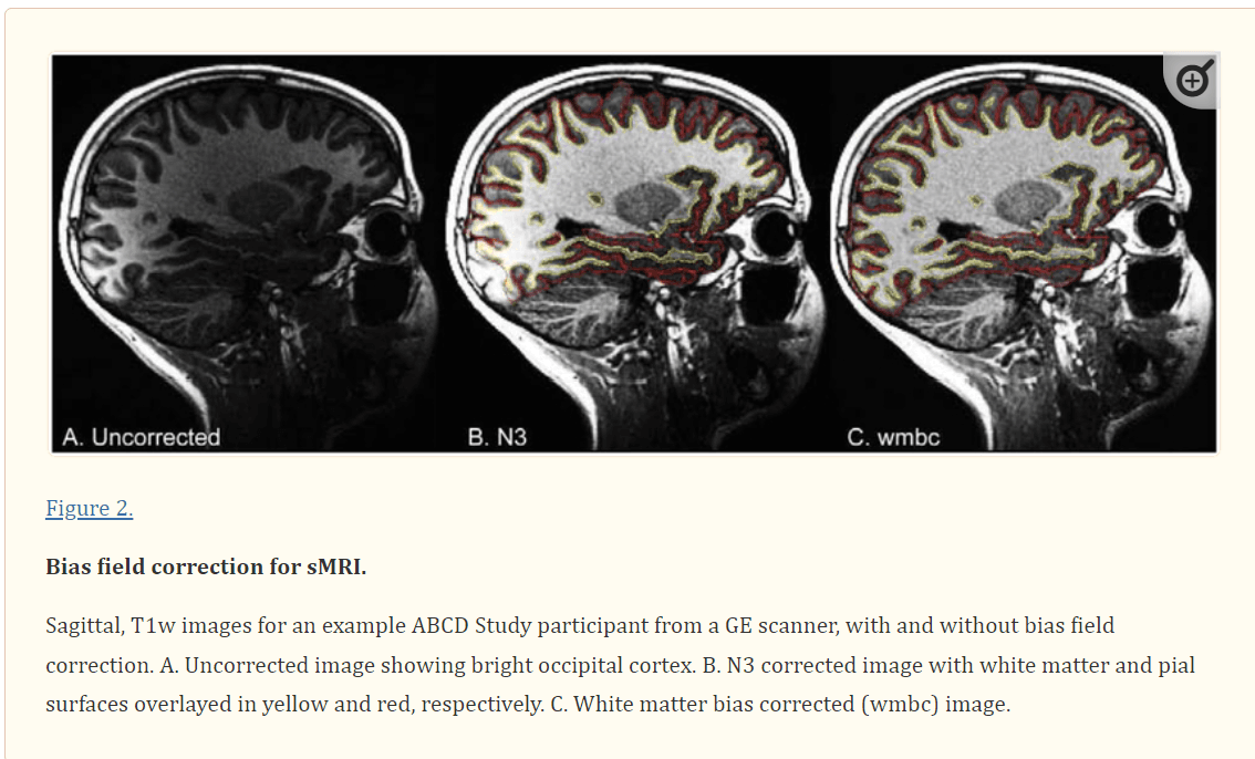
Bias field correction for sMRI. Sagittal, T1w images for an example ABCD Study participant from a GE scanner, with and without bias field correction. A. Uncorrected image showing bright occipital cortex. B. N3 corrected image with white matter and pial surfaces overlayed in yellow and red, respectively. C. White matter bias corrected (wmbc) image.

Intensity inhomogeneity correction is performed by applying smoothly varying, estimated B₁-bias fields, using a novel implementation that is similar in purpose to commonly used bias field correction methods (Ashburner and Friston, 2000; Sled et al., 1998). Specifically, B₁-bias fields are estimated using sparse spatial smoothing and white matter segmentation, with the assumption of uniform T₁w (or T₂w) intensity values within white matter. To normalize T₁w and T₂w intensities across participants, a target white matter intensity value of 110 is used so that after bias correction, white matter voxel intensities are centered on that target value and all other voxels are scaled relatively. The value of 110 was chosen to match the white matter value assigned by the standard bias correction used by FreeSurfer. The white matter mask, defined using a fast, atlas-based, brain segmentation algorithm, is refined based on a neighborhood filter, in which outliers in intensity -- relative to their neighbors within the mask -- are excluded from the mask. A regularized linear inverse, implemented with an efficient sparse solver, is used to estimate the smoothly varying bias field. The stiffness of the smoothing constraint was optimized to be loose enough to accommodate the extreme variation in intensity that occurs due to proximity to the imaging coils, without overfitting local intensity variations in white matter. The bias field is estimated within a smoothed brain mask that is linearly interpolated to the edge of the volume in both directions along the inferior-superior axis, avoiding discontinuities in intensity between brain and neck.

Images are rigidly registered and resampled into alignment with an averaged reference brain in standard space, facilitating standardized viewing and analysis of brain structure. This pre-existing, in-house, averaged, reference brain has 1.0 mm isotropic voxels and is roughly aligned with the anterior commissure / posterior commissure (AC/PC) axis. This standard reference brain was created by averaging T1w brain images from 500 adults after they had been nonlinearly registered to an initial template brain image using discrete cosine transforms (DCT) (Friston et al., 1995). For most ABCD participants, a single scan of each type (T1w or T2w) is collected. If multiple scans of a given type are obtained, only one is used for processing and analysis. Results of manual quality control (QC) performed prior to the full image processing are used to exclude poor-quality structural scans (refer to the Protocol Compliance and Initial Quality Control section). If there is more than one acceptable scan of a given type, the scan with the fewest issues noted is used. In case of a tie, the final acceptable scan of the session is used.

Brain Segmentation

Cortical surface reconstruction and subcortical segmentation are performed using FreeSurfer v5.3, which includes tools for estimation of various measures of brain morphometry and uses routinely acquired T₁w MRI volumes (Dale et al., 1999; Dale and Sereno, 1993; Fischl and Dale, 2000; Fischl et al., 2001; Fischl et al., 2002; Fischl et al., 1999a; Fischl et al., 1999b; Fischl et al., 2004; Segonne et al., 2004; Segonne et al., 2007). The FreeSurfer package has been validated for use in children (Ghosh et al., 2010) and used successfully in large pediatric studies (Jernigan et al., 2016; Levman et al., 2017). Because intensity scaling and inhomogeneity correction are previously applied (see sMRI Preprocessing), the standard FreeSurfer pipeline was modified to bypass the initial intensity scaling and N3 intensity inhomogeneity correction (Sled et al., 1998). As of ABCD Data Release 2.0.1, the T₂w MRI volumes are not used in the cortical surface reconstruction and subcortical segmentation, but this may be incorporated in future releases. Because FreeSurfer 6.0 was formally released after the start of ABCD testing and data acquisition (January 23, 2017), there was not an adequate opportunity to test this new version. Accordingly, ABCD Data Releases 1.0 – 2.0.1 used FreeSurfer version 5.3, and we expect to use FreeSurfer version 6.0 or higher in future ABCD Data Releases.

Subcortical structures are labeled using an automated, atlas-based, volumetric segmentation procedure (Fischl et al., 2002) (Supp. Table 1). Labels for cortical gray matter and underlying white matter voxels are assigned based on surface-based nonlinear registration to the atlas based on cortical folding patterns (Fischl et al., 1999b) and Bayesian classification rules (Desikan et al., 2006; Destrieux et al., 2010; Fischl et al., 2004) (Supp. Tables 2 & 3). Fuzzy-cluster parcellations based on genetic correlation of surface area are used to calculate averages of cortical surface measures for each parcel (Chen et al., 2012) (Supp. Table 4). Functionally-defined parcels, based on resting-state correlations in fMRI (Gordon et al., 2016), are resampled from atlas-space to individual subject-space, and used for resting-state fMRI analysis (Supp. Table 5).

sMRI Morphometric and Image Intensity Analysis

Morphometric measures include cortical thickness (Fischl and Dale, 2000; Rimol et al., 2010), area (Chen et al., 2012; Joyner et al., 2009), volume, and sulcal depth (Fischl et al., 1999a). Image intensity measures include T₁w, T₂w, and T₁w and T₂w cortical contrast (normalized difference between gray and white matter intensity values) (Westlye et al., 2009). Cortical contrast measures are included because they reflect factors that impact placement of the gray-white matter boundary, such as pericortical myelin content, that can significantly influence cortical thickness measures. Cortical contrast has also been shown to have unique genetic influences (Panizzon et al., 2012), and may be a more sensitive cortical marker when examining questions related to brain development (Lewis et al., 2018) and psychopathology (Norbom et al., 2018). We sample intensity values at a distance of ±0.2 mm -- relative to the gray-white boundary -- along the normal vector at each surface location and calculate cortical contrast from gray and white matter values ( [white - gray] / [white + gray] / 2). We calculate averages for each cortical parcel in the two standard FreeSurfer parcellation schemes (Desikan et al., 2006; Destrieux et al., 2010) using unsmoothed, surface-based maps of morphometric and image intensity measures. For each of the fuzzy-cluster parcels (Chen et al., 2012), we calculate weighted averages (weighted by fuzzy cluster membership values ranging from 0 to 1) for each measure using smoothed surface maps (~66 mm FWHM, matching the level of smoothing used for derivation of the fuzzy cluster parcels). We also calculate averages of the unsmoothed intensity measures for the volumetric subcortical ROIs, in addition to the volume of each structure.

Post-processed sMRI Quality Control

To ensure the quality of derived measures, trained technicians review the accuracy of cortical surface reconstruction. For each cortical surface reconstruction, reviewers gauge the severity of five categories of image artifact or reconstruction inaccuracy: motion, intensity inhomogeneity, white matter underestimation, pial overestimation, and magnetic susceptibility artifact. Numeric values are assigned on a scale of 0–3, indicating absent, mild, moderate, and severe levels of each type of artifact, respectively. The reviewers assign an overall QC score indicating whether the cortical surface reconstruction is recommended for use (1) or recommended for exclusion (0). Exclusion is recommended if any of the five categories are rated as severe (a value of 3).

dMRI Processing and Analysis

dMRI Preprocessing

Eddy current correction (ECC) uses a model-based approach, predicting the pattern of distortions across the entire set of diffusion weighted volumes, based on diffusion gradient orientations and amplitudes (Zhuang et al., 2006), with corrections limited to displacement along the phase-encode direction (Andersson and Sotiropoulos, 2016; Barnett et al., 2014; Rohde et al., 2004; Zhuang et al., 2006). With a total of 12 free parameters across the entire set of volumes, we model displacements in the phase encode direction as functions of spatial location, gradient orientation, and gradient strength. Because abrupt head motion often results in severe signal loss in individual slices for a particular frame, we use a robust tensor fit to exclude these dark slices so that they do not influence the estimation of eddy current distortions. To identity these dark slices, we first use standard linear estimation of tensor model parameters from log transformed images (Basser et al., 1994a). The RMS of the residual error for each frame of each slice is calculated across brain voxels and then normalized by the median RMS value across frames within a given slice. For a given slice, frames with normalized RMS greater than 3.2 are censored from subsequent tensor fits, resulting in a tighter fit for the non-censored frames. A total of three iterations are sufficient to settle upon a stable tensor fit excluding dark frames for a given slice (frame-slices). To prevent dark frame-slices from influencing the estimation of eddy current distortions, such frames are replaced (for a given slice) with the corresponding image synthesized from the censored tensor fit. ECC is optimized using Newton’s method through minimization of RMS error between each eddy-current-corrected image and the corresponding image synthesized from the censored tensor fit, accounting for image contrast variation between frames. After applying corrections for the estimated distortions, we re-estimate the tensor, again excluding the dark frame-slices identified earlier, to produce a more accurate template for subsequent iterations of ECC, with five iterations in total.

To correct images for head motion, we rigid-body-register each frame to the corresponding volume synthesized from the post-ECC censored tensor fit. We remove the influence of dark frame-slices from motion correction and future analysis by replacing those images with values interpolated from the tensor fit calculated without their contribution. The diffusion gradient matrix is adjusted for head rotation, important for accurate model fitting and tractography (Hagler et al., 2009; Leemans and Jones, 2009). Mean head motion values (average FD) are calculated and made available for possible use as covariates in group-level statistical analyses to account for residual effects (Yendiki et al., 2013).

Spatial and intensity distortions caused by B₀ field inhomogeneity are minimized using a robust and accurate procedure for reducing spatial and intensity distortions in EPI images that relies on reversing phase-encode polarities (Andersson et al., 2003; Chang and Fitzpatrick, 1992; Holland et al., 2010; Morgan et al., 2004). Pairs of b=0 (i.e., non-diffusion weighted) images with opposite phase encoding polarities (and thus opposite spatial and intensity distortion patterns) are aligned using a fast, nonlinear registration procedure, and the estimated displacement field volume is used to correct distortions in each frame (successive diffusion-weighted volumes) (Holland et al., 2010). Gradient nonlinearity distortions are then corrected for each frame (Jovicich et al., 2006). The b=0 dMRI images are registered to T₁w structural images using mutual information (Wells et al., 1996) after coarse pre-alignment via within-modality registration to atlas brains. dMRI images are then resampled with 1.7 mm isotropic resolution (equal to the dMRI acquisition resolution), with a fixed rotation and translation relative to the corresponding T₁w image that has been rigidly resampled into alignment with an atlas brain. This provides a standard orientation for the resulting dMRI images, fitting the brain within the set of axial dMRI slices and producing more consistent diffusion orientations across participants, as viewed with diffusion encoded color (DEC) fractional anisotropy (FA) map images. The diffusion gradient matrix is again adjusted for head rotation. Cubic interpolation is used for each of these resampling steps. A registration matrix is provided to specify the rigid-body transformation between dMRI and T₁w images.

Fiber Tract Segmentation

Major white matter tracts are labelled using AtlasTrack, a probabilistic atlas-based method for automated segmentation of white matter fiber tracts (Hagler et al., 2009). The fiber atlas contains prior probabilities and orientation information for specific long-range projection fibers, including some additional fiber tracts not included in the original description (Hagler et al., 2009), such as cortico-striate connections and inferior to superior frontal cortico-cortical connections (Supp. Table 6). sMRI images for each subject are nonlinearly registered to the atlas using discrete cosine transforms (DCT) (Friston et al., 1995), and diffusion tensor imaging (DTI)-derived diffusion orientations for each subject are compared to the atlas fiber orientations, refining the a priori tract location probabilities, individualizing the fiber tract ROIs, and minimizing the contribution from regions inconsistent with the atlas. Voxels containing primarily gray matter or cerebral spinal fluid, identified using FreeSurfer’s automated brain segmentation (Fischl et al., 2002), are excluded from analysis.

dMRI Microstructural Analysis

We calculate several standard measures related to microstructural tissue properties using DTI (Basser et al., 1994b; Basser and Pierpaoli, 1996), including FA and mean, longitudinal (or axial), and transverse (or radial) diffusivity (MD, LD, and TD) (Alexander et al., 2007). Diffusion tensor parameters are calculated using a standard, linear estimation approach with log-transformed diffusion-weighted (DW) signals (Basser et al., 1994a). We calculate two different tensor model fits. In the first DTI model fit (DTI inner shell, or DTI_IS), frames with b>1000 s/mm² are excluded from tensor fitting (leaving 6 directions at b=500 s/mm² and 15 directions at b=1000 s/mm²) so that the derived diffusivity measures better correspond to those from traditional, single-b-value acquisitions. In the second DTI model fit (DTI full shell, or DTI_FS), we include all gradient strengths/shells (6 directions at b=500 s/mm², 15 directions at b=1000 s/mm², 15 directions at b=2000 s/mm², and 60 directions at b=3000 s/mm²).

Taking advantage of the multiple b-value acquisition, we also fit a Restriction Spectrum Imaging (RSI) model (White et al., 2013a; White et al., 2014; White et al., 2013b), a linear estimation approach that allows for mixtures of “restricted” and “hindered” diffusion within individual voxels. We use RSI to model two volume fractions, representing intracellular (restricted) and extracellular (hindered) diffusion, with separate fiber orientation density (FOD) functions, modeled as fourth order spherical harmonic functions, allowing for multiple diffusion orientations within a single voxel. For both fractions, LD is held constant, with a value of 1×10⁻³ mm²/s. For the restricted fraction, TD is modelled as 0. For the hindered fraction, TD is modelled as 0.9 × 10⁻³ mm²/s. Measures derived from this RSI model fit (summarized in Supp. Table 7) include the following: restricted normalized isotropic (N0), restricted normalized directional (ND), restricted normalized total (NT), hindered normalized isotropic (N0_s2), hindered normalized directional (ND_s2), and hindered normalized total (NT_s2). Each of these measures is defined as the Euclidean norm (square root of the sum of squares) of the corresponding model coefficients divided by the norm of all model coefficients. These normalized RSI measures are unitless and range from 0 to 1. The square of each of these measures is equivalent to the signal fraction for their respective model components. N0 and NT_s2 are derived from the 0th order spherical harmonic coefficients of the restricted and hindered fractions, respectively, and reflect varying contributions of intracellular and extracellular spaces to isotropic diffusion-related signal decreases in a given voxel. ND and ND_s2 are calculated from norm of the 2nd and 4th order spherical harmonic coefficients of the restricted and hindered fractions, respectively. These higher order components reflect oriented diffusion; diffusion that is greater in one orientation than others. Qualitatively, ND is very similar to FA, except that, by design, it is unaffected by crossing fibers. NT and NT_s2 reflect the overall contribution to diffusion signals of intracellular and extracellular spaces, and are calculated from the norm of the 0th, 2nd, and 4th order coefficients of the restricted and hindered fractions, respectively, again divided by the norm of all model coefficients.

Mean DTI and RSI measures are calculated for white matter fiber tract ROIs created with AtlasTrack (Hagler et al., 2009) and for ROIs derived from FreeSurfer’s automated subcortical segmentation (Fischl et al., 2002). With fiber tracts represented as thresholded probability maps, probability estimates are used to calculate weighted averages of DTI and RSI measures. DTI and RSI measures are also sampled onto the FreeSurfer-derived cortical surface mesh to make maps of diffusion properties for cortical gray matter and white matter adjacent to the cortex (Govindan et al., 2013; Kang et al., 2012) and calculate surface-based ROI averages for the anatomical, cortical parcellations (Desikan et al., 2006; Destrieux et al., 2010). Values are sampled with linear interpolation perpendicular to the gray/white boundary (“white” surface) in 0.2 mm increments, ranging from 0.8–2 mm in both directions. White and gray matter values are calculated by combining samples within tissue type using a weighted average based on the proportion of white or gray matter in each voxel (Elman et al., 2017). For subcortical ROIs, contamination due to partial voluming in the ROI with CSF is suppressed by calculating weighted averages. Specifically, weighting factors for each voxel in the ROI are calculated based on the difference of MD values relative to the median within each ROI. The typical dispersion of MD values is defined for each ROI as the median absolute deviation from the median (MAD), averaged across subjects. Weighting factors are calculated using Tukey’s bisquare function such that lower weights are assigned to voxels with MD values farther from the median value, relative to the dispersion values multiplied by 4.7 (Tukey, 1960).

Post-processed dMRI Quality Control

For the subset of participants included in ABCD Data Release 1.1, dMRI data were visually inspected after processing. Time permitting, dMRI data for the remaining participants may be similarly reviewed and their results included in a future patch release. Reviewers compare RSI-derived ND images (see dMRI Microstructural Analysis) to corresponding, co-registered T₁w images, and rate each dMRI series along five dimensions of quality: residual B₀ distortion, registration to the T₁w image, image quality, segmentation integrity, and field of view (FOV) cutoff. For each, numeric values of 0–3 are assigned, indicating absent, mild, moderate, and severe. Residual distortion is assessed by looking for stretching or compression of white matter tracts in the ND image relative to the rigid-body co-registered T₁w image, focusing on the corpus callosum and frontal lobe. Poor registration is rated on the basis of visible rotation or translation between the T₁w and RSI-ND images. The image quality rating is based on the presence of banding, graininess, motion, artifacts, or poor gray/white contrast in the ND image. The automatic white matter tract segmentation is assessed for incompleteness, absence, or gross mis-location. FOV cutoff indicates clipping of the dorsal or ventral aspect of the cortex. Each dMRI series is then assigned an overall QC score of recommended for use (1) or recommended for exclusion (0). A series will be recommended for exclusion (QC score of 0) if B₀ warp, registration, image quality, or segmentation are rated as severe (a value of 3). While FOV cutoff is assessed, it is not used as a factor in deciding the overall QC score.

fMRI Processing and Analysis

fMRI Preprocessing

Head motion is corrected by registering each frame to the first using AFNI’s 3dvolreg (Cox, 1996), which also provides estimates of head motion time courses that are incorporated into task-fMRI and resting-state-fMRI single-subject analyses (see below). B₀ distortions are corrected using the same reversing polarity method used for the dMRI (Holland et al., 2010). To avoid signal “drop-out” due to within-voxel field gradients in gradient-echo acquisitions, the displacement field is estimated from separate spin-echo calibration scans, then adjusted for estimated between-scan head motion, and finally applied to the series of gradient-echo images. Images are next corrected for distortions due to gradient nonlinearities (Jovicich et al., 2006). To correct for between-scan motion, each scan is resampled with cubic interpolation into alignment with a reference scan that is chosen as the one nearest to the middle of the set of fMRI scans for a given participant. The alignment is based on rigidly-registering the first frame of each scan to the first frame of the reference scan. Automated registration between the spin-echo, B₀ calibration scans (i.e., field maps) and T₁w structural images is performed using mutual information (Wells et al., 1996) with coarse pre-alignment based on within-modality registration to atlas brains. A registration matrix is provided to specify the rigid-body transformation between fMRI and T1w images. The resulting fMRI images remain in “native-space” and have 2.4 mm isotropic resolution.

Task-fMRI Behavioral Measures

Behavioral measures specific to each task are calculated to assess performance and identify participants with poor accuracy or slow reaction times (Casey et al., 2018). MID: With three types of trials, participants have a chance to either win money, lose money, or earn nothing. Wins and losses are further subdivided into small and large magnitudes. After a short response time window, positive or negative feedback informs the participant about performance in each trial. Behavioral metrics for each trial type include: number of trials, mean and standard deviation (SD) of reaction times to the different incentive magnitudes, and total monetary earning. Poor performance is indicated by a behavioral performance flag variable if any trial type across both runs yields less than 4 events in either the positive or negative feedback. SST: On “Go” trials, participants indicate by button press, during a short response time window, whether an arrow presented points leftward or rightward. On less frequent “Stop” trials, a delayed stop signal is presented, instructing the participant to withhold the motor response. The primary categories of trial-response combinations are “Correct Go”, “Incorrect Go”, “Correct Stop”, and “Incorrect Stop”3. For each category, behavioral metrics include: number of trials, mean and SD of reaction times, mean stop signal delay, and mean stop signal reaction time. Poor performance is indicated if: number of Go trials <50, Correct Go percentage <60%, Incorrect Go >30%, Late Go (both correct and incorrect) >30%, No Response Go >30%, number of Stop trials <30, Stop trial accuracy <20% or >80%, or Correct Go Reaction Time (RT) < Incorrect Stop RT. EN-Back: With a block design of 0-back and 2-back working memory tasks, participants indicate by button press the repeated presentation of images. Image types include emotionally positive, negative, or neutral faces or pictures of places. Behavioral metrics include: total number of trials presented, number of correct responses, and accuracy (correct responses divided by total trials), and mean and SD of reaction times for correct responses. Following the imaging session, the EN-Back Recognition Memory task asks the participant to decide if pictures presented were seen previously in the EN-Back task. For each stimulus type (old and new), hit rates and false alarm rates are calculated. Additional metrics include corrected accuracy (hit rate from working memory task minus false alarm rate from recall task), response bias, and d-prime. Poor performance is indicated if the overall response accuracy for the 0-back or 2-back blocks is less than 60%.

Task-fMRI Analysis

Estimates of task-related activation strength are computed at the individual subject level using a general linear model (GLM) and an ROI-based approach.

Pre-analysis processing: Processing steps subsequent to fMRI preprocessing include the removal of initial frames4 to ensure equilibration of the T₁w signal and normalization of voxel time series by dividing by the mean across time of each voxel. Surface sampling: Preprocessed time courses are sampled onto the cortical surface for each individual subject. Voxels containing cortical gray matter are projected onto the surface by sampling values 1 mm from the gray/white boundary, into cortical gray matter, along the surface normal vector at each vertex (using FreeSurfer’s mri_vol2surf with “white” surface, “-projdist 1” option, and default “nearest” interpolation). ROI values extraction: Average time courses are calculated for cortical surface-based ROIs using FreeSurfer’s anatomically-defined parcellations (Desikan et al., 2006; Destrieux et al., 2010) and subcortical ROIs (Fischl et al., 2002).

Nuisance regressors:

Baseline and quadratic trends in the time-series data are included in the analysis. Motion estimates and their derivatives are also included as regressors (Power et al., 2014). Time points with FD greater than 0.9 mm are censored (Siegel et al., 2014). Estimated motion time courses used for regression and censoring are temporally filtered using an infinite impulse response (IIR) notch filter to attenuate signals in the range of 0.31 – 0.43 Hz. This frequency range corresponds to empirically observed oscillatory signals in motion estimates linked to respiration and the dynamic changes in magnetic susceptibility due to lung movement in the range of 18.6 – 25.7 respirations / minute. With the removal of these fast oscillations linked to respiration, the filtered motion estimates and FD values more accurately reflect actual head motion (Fair et al., 2018).

General linear model:

Estimates of task-related activation strength are computed at the individual subject level using a general linear model (GLM) implemented in AFNI’s 3dDeconvolve (Cox, 1996). Hemodynamic response functions are modelled with two parameters using a gamma variate basis function plus its temporal derivative (using AFNI’s ‘SPMG’ option within 3dDeconvolve). Task models include stimulus timing for each condition and linear contrasts of conditions (see Supp. Tables 8–10). For MID and SST analyses, events are modeled as instantaneous; for EN-back, the duration of cues (~3 s) and trial blocks (~24 s) are modeled as square waves convolved with the two parameter gamma basis function (i.e., block duration specified when using AFNI’s ‘SPMG’ option). Outputs include GLM beta coefficients and standard errors of the mean (SEM; calculated from the ratio of the beta and t-statistic) calculated for each voxel, vertex, or ROI time series.

Averaging across runs: ROI average beta coefficients and standard errors are computed for each of two runs. We compute the average across runs for each participant weighted by the nominal degrees of freedom (number of frames remaining after motion censoring minus number of model parameters, but not accounting for temporal autocorrelation), which differs between runs due to motion censoring. Runs with fewer than 50 degrees of freedom are excluded from the average between runs.

Censoring invalid contrasts:

The frequency and magnitude of head movements varies widely in children. Some participants exhibit frequent periods of motion resulting in greatly reduced numbers of time points used to estimate model parameters. Depending on when supra-threshold head movements (FD>0.9 mm) occur relative to instances of a given event type, rare conditions may be under-represented in some participants, or lack representation entirely. For unrepresented conditions, beta and SEM values are undefined and shared as empty cells in the tabulated data. If conditions are under-represented, the design matrix of the GLM analysis becomes ill-conditioned, making estimated beta weights unreliable for those conditions and the contrasts that include them. In rare cases, this results in extreme values for the beta and SEM estimates, as much as several orders of magnitude different from typical values for a given contrast. The presence of extreme outliers violates standard parametric assumptions, so group-level statistical analyses can produce invalid and nonsensical results. To prevent this, we censor the beta and SEM values if they are identified as having extremely high SEM values and therefore low reliability beta estimates. For a given subject with an extreme value for a particular contrast and ROI, there are typically outliers in other brain regions for the same subject and contrast and generally greater variation across brain regions. We censor the beta and SEM values for all ROIs for those contrasts that have RMS of SEM values across the cortical surface greater than 5% signal change. This represents less than 0.5% of all subject-task-contrast-run combinations. The censored values are replaced with empty cells.

Resting-State fMRI Analysis

Measures of functional connectivity are computed using a seed-based, correlational approach (Van Dijk et al., 2010), adapted for cortical surface-based analysis (Seibert and Brewer, 2011). Pre-analysis processing: Pre-analysis processing steps, which are not part of the fMRI preprocessing, include the removal of initial frames, normalization, regression, temporal filtering, and calculation of ROI-average time courses. After removing the initial frames4, we normalize voxel time series by dividing by the mean across time of each voxel and then use linear regression to remove quadratic trends, signals correlated with estimated motion time courses, and the mean time courses of cerebral white matter, ventricles, and whole brain, as well as their first derivatives (Power et al., 2014; Satterthwaite et al., 2012). The white matter, ventricle, and whole brain ROIs used to calculate mean time courses were derived from FreeSurfer’s automated brain segmentation (aseg), resampled into voxel-wise alignment with the fMRI data, and then eroded by a single fMRI-resolution voxel. Motion regression includes six parameters plus their derivatives and squares. As described above for task fMRI analysis, estimated motion time courses are temporally filtered to attenuate signals linked to respiration. Frames with displacement (FD) greater than 0.3 mm are excluded from the regression (Power et al., 2014). After regression, time courses are band-pass filtered between 0.009 and 0.08 Hz (Hallquist et al., 2013).

Surface sampling and ROI averaging:

Preprocessed time courses are sampled onto the cortical surface for each individual subject in the same manner as the task-fMRI data. Average time courses are calculated for cortical surface-based ROIs using FreeSurfer’s anatomically-defined parcellations (Desikan et al., 2006; Destrieux et al., 2010) and a functionally-defined parcellation based on resting-state functional connectivity patterns (Gordon et al., 2016) that are resampled from atlas-space to individual subject-space. Average time courses are also calculated for subcortical ROIs (Fischl et al., 2002). Variance across time is calculated for each ROI, a measure that reflects the magnitude of low frequency oscillations.

Network correlation analysis:

We calculate correlation values for each pair of ROIs, which are Fisher transformed to z-statistics and averaged within or between networks to provide summary measures of network correlation strength (Van Dijk et al., 2010). Within the Gordon parcellation, ROIs are grouped together into several networks (e.g., default, fronto-parietal, dorsal attention, etc.) (Gordon et al., 2016) (Supp. Table 5). Average correlation within a network is calculated as the average of the Fisher-transformed correlations for each unique, pairwise combination of ROIs belonging to that network. Average correlation between one network and another is calculated similarly by averaging the correlations for each unique, pairwise combination of ROIs in the first network with the ROIs in the second. In addition, we calculate the correlation between each network and each subcortical gray matter ROI by averaging the correlations between each ROI in the network and a given subcortical ROI.

Motion censoring:

Motion censoring is used to reduce residual effects of head motion that may survive the regression (Power et al., 2012; Power et al., 2014). Time points with FD greater than 0.2 mm are excluded from the variance and correlation calculations. Note that this is a slightly more conservative threshold than that used for the regression step. Time periods with fewer than five contiguous, sub-threshold time points are also excluded. The effects of head motion can potentially linger for several seconds after an abrupt head motion, for example due to spin-history or T₁ relaxation effects (Friston et al., 1996), so an additional round of censoring is applied based on detecting time points that are outliers with respect to spatial variation across the brain. SD across ROIs is calculated for each time point, and outlier time points, defined as having an SD value more than three times the median absolute deviation (MAD) below or above the median SD value, are excluded from variance and correlation calculations. Averaging across runs: ROI variance and network correlation values are averaged across rs-fMRI runs, weighted by the number of frames per run remaining after motion censoring. Runs with fewer than 100 usable time points (out of 375 acquired) are excluded from the average. Participants with no usable runs receive empty values in the tabulated results.

Post-processed fMRI Quality Control

For ABCD Data Release 2.0.1, only automated and manual QC of fMRI data was performed as detailed above. The DAIC and partners are currently investigating optimal post-processed fMRI reviews, which would resemble in part the post-processed dMRI QC procedure.

Data and Methods Sharing

Public sharing of unprocessed, preprocessed, and derived imaging data is undertaken in partnership with the NDA (https://data-archive.nimh.nih.gov/abcd). DICOM files are made publicly available via a “Fast Track” mechanism on a continual basis within approximately one month of data collection. Preprocessed NIfTI files and tabulated results of ROI-based analyses are shared in annual data releases. This manuscript documents the methods shared as part of the second annual release, ABCD Data Release 2.0, which was made available in March 2019 and includes results for the complete 2016–2018 baseline sample. The data presented here combines the ABCD Data Release 2.0 with the amended ABCD Fix Release 2.0.1 data release July 2019. We have packaged the processing pipeline described here within a portable container format (Docker container), which includes a lightweight, virtualized Linux environment and the complete execution environment, including all required software dependencies. Users may currently download a beta-testing version of the executable Docker container from NITRC (https://www.nitrc.org/projects/abcd_study).

Results

The imaging-derived, tabulated data included in ABCD Release 2.0.1 is a rich set of measures sampled from multiple imaging modalities and anatomical regionalization schemes from a large, diverse sample of children aged 9–10 (n = 11759 underwent an MRI exam). For individual participants, some scans may have been omitted from the standard imaging protocol due to fatigue and/or time constraints. The identification of severe imaging artifacts during our initial QC leads to the exclusion of additional series. In Figures 3 and ​4, flow charts illustrate sources of data loss that reduce the numbers of participants available for analyses using the tabulated data from each modality. Red boxes show the primary exclusions that prevent us from running either the required processing or analysis steps. White boxes represent the tabulated data for each modality. Additional data loss at this stage reflects participants for whom results were excluded from the curated dataset for various reasons. In rare cases, this was due to miscellaneous processing failures that may be recoverable with additional investigation and intervention. For task fMRI, missing results are related to the exclusion of participants for whom stimulus/response timing files were corrupted, had time stamps inconsistent with the fMRI data acquisition, or had other irregularities in data acquisition, and the censoring of results with high RMS SEM values. For rs-fMRI, missing results reflect the lack of usable scans with an adequate number of valid time points after motion censoring. Through future modification of processing or analysis software and parameters, results for some of the currently excluded participants may be recoverable for future data releases. Finally, the blue boxes represent the optional filtering steps specified in our recommended inclusion criteria (Supp. Table 11).

Figure 3.

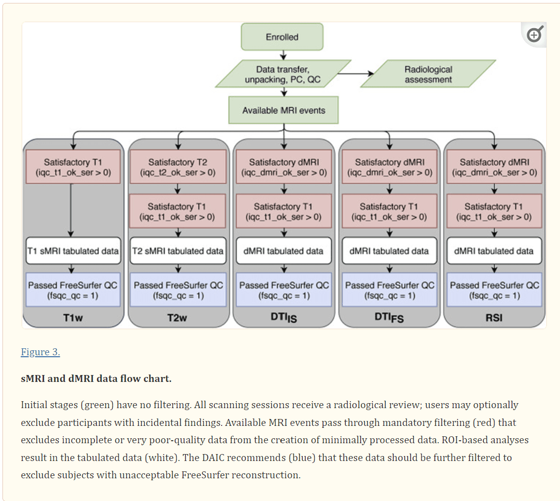
sMRI and dMRI data flow chart. Initial stages (green) have no filtering. All scanning sessions receive a radiological review; users may optionally exclude participants with incidental findings. Available MRI events pass through mandatory filtering (red) that excludes incomplete or very poor-quality data from the creation of minimally processed data. ROI-based analyses result in the tabulated data (white). The DAIC recommends (blue) that these data should be further filtered to exclude subjects with unacceptable FreeSurfer reconstruction.

Figure 4.

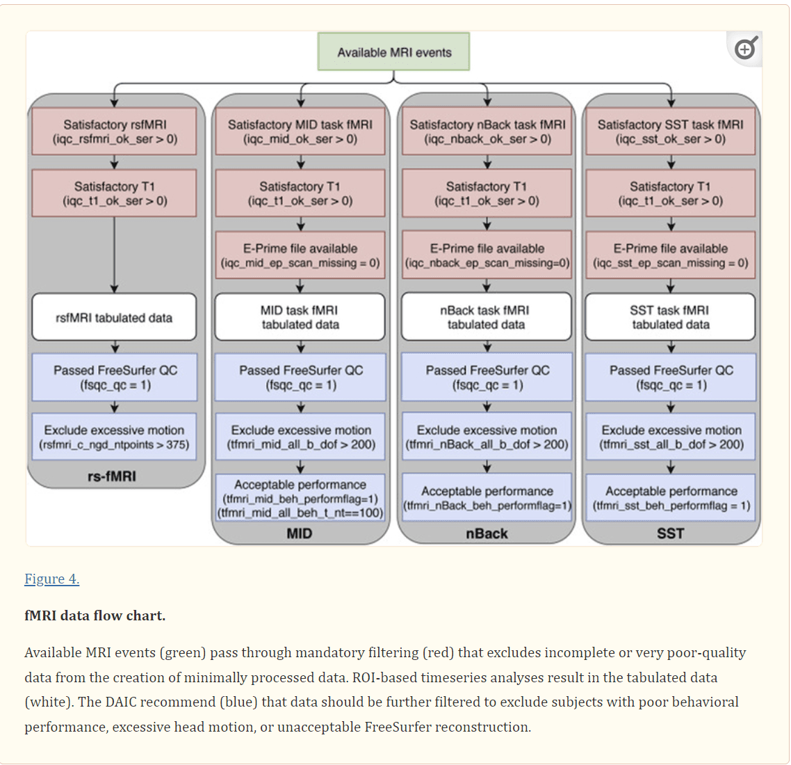
fMRI data flow chart. Available MRI events (green) pass through mandatory filtering (red) that excludes incomplete or very poor-quality data from the creation of minimally processed data. ROI-based timeseries analyses result in the tabulated data (white). The DAIC recommend (blue) that data should be further filtered to exclude subjects with poor behavioral performance, excessive head motion, or unacceptable FreeSurfer reconstruction.

We anticipate that future reports from investigators both within the ABCD consortium and among the greater scientific community will provide comprehensive and detailed characterizations of the baseline dataset included in ABCD Release 2.0.1. Here, we will show preliminary results of a technical survey of this data, focusing on a small set of selected measures from each modality and how they differ among scanner manufacturers (see Supplementary Information for description of analysis methods). Despite efforts to standardize the imaging protocols across platforms, we find between-manufacturer differences that vary in magnitude across modalities and measures. Mean cortical thickness, total cortical area, and T1w gray/white contrast are among the sMRI measures whose group means differ between scanner manufacturers (Fig. 5A–C). dMRI-derived measures from DTI and RSI analyses also vary between manufacturers (Fig. 5D–F). The voxelwise smoothness and tSNR of fMRI data varies by manufacturer, as do task-related activations measured with the EN-back task (Fig. 5G–I). For rs-fMRI, mean motion varies slightly by manufacturer, resulting in varying numbers of usable time points after censoring; within-network correlation strengths also vary (Fig. 5J–L). Because of these differences in each modality, and because of potential differences between individual scanners from a given manufacturer, we recommend that group analyses use the unique identifier for each scanner (i.e., DeviceSerialNumber, mri_info_deviceserialnumber) as a categorical covariate to account for between-scanner variations (Brown et al., 2012), or that similar, statistical harmonization procedures be used.

Figure 5.

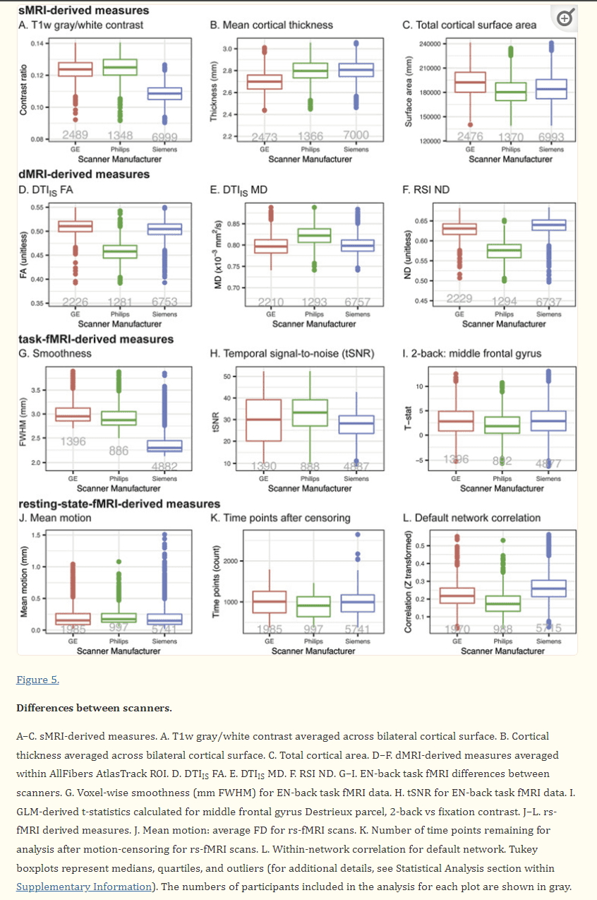
Differences between scanners. A–C. sMRI-derived measures. A. T1w gray/white contrast averaged across bilateral cortical surface. B. Cortical thickness averaged across bilateral cortical surface. C. Total cortical area. D–F. dMRI-derived measures averaged within AllFibers AtlasTrack ROI. D. DTI_IS FA. E. DTI_IS MD. F. RSI ND. G–I. EN-back task fMRI differences between scanners. G. Voxel-wise smoothness (mm FWHM) for EN-back task fMRI data. H. tSNR for EN-back task fMRI data. I. GLM-derived t-statistics calculated for middle frontal gyrus Destrieux parcel, 2-back vs fixation contrast. J–L. rs-fMRI derived measures. J. Mean motion: average FD for rs-fMRI scans. K. Number of time points remaining for analysis after motion-censoring for rs-fMRI scans. L. Within-network correlation for default network. Tukey boxplots represent medians, quartiles, and outliers (for additional details, see Statistical Analysis section within Supplementary Information). The numbers of participants included in the analysis for each plot are shown in gray.

Discussion

The ABCD Study will provide the most comprehensive longitudinal investigation to date of the neurobiological trajectories of brain and behavior development from late childhood through adolescence to early adulthood. There are many risk processes during adolescence that lead to chronic diseases in later life, including tobacco use, alcohol and illicit substance use, unsafe sex, obesity, sports injury and lack of physical activity (Patton et al., 2017). Furthermore, this developmental period can give rise to many common psychiatric conditions including anxiety disorders, bipolar disorder, depression, eating disorders, psychosis, and substance abuse (Hafner et al., 1989; Kessler et al., 2005). The ABCD Study is well-positioned to capture the behavioral and neurobiological changes taking place during healthy development, prodromal behavioral issues, experimentation with drugs and alcohol, and antecedent neuroanatomical changes. Identifying neuropsychological, structural and functional measures as potential biomarkers of psychiatric, neurological and substance abuse disorders may better inform the diagnosis and treatment of youth who present with early mental and physical health concerns.

Rigorous acquisition monitoring and uniform image processing of a large cohort of ethnically diverse young people regularly over adolescence is necessary to characterize subtle neuroanatomical and functional changes during such a plastic developmental period. Curated ABCD Data Releases providing canonical neuroimaging measures for this large dataset will enable the scientific community to test innumerable hypotheses related to brain and cognitive development. Meanwhile, the DAIC and ABCD collaborators will continue working to improve and extend the image processing pipeline, resulting in new and evolving imaging metrics to be evaluated for potential inclusion in future, curated ABCD Data Releases. Considering these novel metrics alongside canonical measurements provides the ability to compare and contrast new and existing analytical techniques. The capability to regularly reprocess all data for new analytic pipelines is made possible by the framework described in this manuscript. The intent is for the methods developed here to be shareable and deployable for other large-scale neuroimaging studies.

Limitations and Caveats

On an ongoing basis, the Fast Track data sharing mechanism occurs shortly after data collection, without processing, quality control, or curation, and includes all ABCD imaging data available and permitted to be shared. Imaging series with the most severe artifacts or those with missing or corrupted DICOM files are excluded from subsequent processing, and so are not included in the minimally processed or tabulated data sharing. For a given modality, additional participants may be missing from the tabulated data due to failures in brain segmentation or modality-specific processing and analysis. However, successfully processed data with moderate imaging artifacts are included in the minimally processed and tabulated data sharing. This is necessary to enable certain studies, such as methodological investigations of the effect of imaging artifacts on derived measures. For most group analyses, we recommend excluding cases with significant incidental findings, excessive motion, or other artifacts, and we provide a variety of QC-related metrics for use in applying sets of modality-specific, inclusion criteria (Supp. Table 11; see NDA Annual Release 2.0.1 Notes ABCD Imaging Instruments for additional details). Some researchers may wish to use this as a template for customized inclusion criteria that could include additional QC metrics or apply more conservative thresholds.

While Fast Track provides early access to DICOM data, this comes with the caveat that users may process the data inappropriately, resulting in inaccurate or spurious findings. The purpose of the ABCD processing pipeline is to provide images and derived measures for curated ABCD Data Releases using consensus-derived approaches for processing and analysis. Since the processing pipeline is expected to change over time, we suggest that authors clearly state the version of the release used (e.g., Adolescent Brain Cognitive Development Study (ABCD) - Annual Release 2.0, DOI: 10.15154/1503209). Each new release documents changes and includes data provided in previous releases, reprocessed as necessary to maintain consistency within a particular release. Combining data between curated Data Releases is not recommended, but Fix Releases partially replace some of the previous Data Release that was found to be erroneous (ABCD Fix Release 2.0.1, DOI: 10.15154/1504041).

Future Directions

Mirroring the general progression of neuroimaging processing tools and analysis methods in the field, the processing pipeline used for future ABCD Data Releases is expected to evolve over time. We must consider future challenges specific to longitudinal analyses, such as the possibility of scanner and head coil upgrade or replacement during the period of study. Also, other image analysis methods, either recently developed or soon to be developed, may better address particular issues, perhaps by providing superior correction of imaging artifacts, more accurate brain segmentation, or additional types of biologically relevant, imaging-derived measures. For example, FreeSurfer’s subcortical segmentation pipeline in its current implementation exhibits some bias, both with under- and over-estimation of particular structures, compared to the gold standard of manual segmentation (Makowski et al., 2018; Schoemaker et al., 2016). Furthermore, there are a variety of excellent neuroimaging toolboxes available for preprocessing of dMRI data, such as FSL (Smith et al., 2004), TORTOISE (Irfanoglu et al., 2017; Pierpaoli et al., 2010), and DTIprep (Oguz et al., 2014), that use similar approaches but varied implementations to address the major challenges. Within the ABCD consortium, efforts are underway to process ABCD data using alternative approaches for various stages of processing or analysis to compare methods using quantitative metrics of the reliability of the derived results. In addition, results of processing ABCD data with a modified version of the HCP pipeline (Glasser et al., 2013) are planned for future public release. In general, we seek to enhance and augment ABCD image analysis over time by incorporating new methods and approaches as they are implemented and validated.

To enable researchers to more easily take advantage of this data resource, the DAIC provides a web-based tool called the ABCD Data Exploration and Analysis Portal (DEAP, updated shortly after Data Releases). This tool provides convenient access to the complete battery of ROI-based, multimodal imaging-derived measures as well as sophisticated statistical routines using generalized additive mixed models to analyze repeated measures and appropriately model the effects of site, scanner, family relatedness, and a range of demographic variables. Future releases will also support voxel-wise (volumetric) and vertex-wise (surface-based) analyses.

As a ten-year longitudinal study with participants returning every two years for successive waves of imaging, future ABCD Data Releases will include multiple time points for each participant. All imaging-derived measures provided for the baseline time point will also be generated independently for each successive time point. In addition, within-subject, longitudinal analyses will provide more sensitive estimates of longitudinal change for some imaging measures. For example, the FreeSurfer longitudinal processing stream reduces variability and increases sensitivity in the measurement of changes in cortical thickness and the volumes of subcortical structures (Reuter and Fischl, 2011; Reuter et al., 2010; Reuter et al., 2012). Analyses of cortical and subcortical changes in volume with even greater sensitivity is available through Quantitative Analysis of Regional Change (QUARC) (Holland et al., 2009; Holland and Dale, 2011; Holland et al., 2012; Thompson and Holland, 2011). A variant of QUARC is also available for longitudinal analysis of dMRI data with improved sensitivity (McDonald et al., 2010). The goal of future development and testing will be to provide a collection of longitudinal change estimates for a variety of imaging-derived measures that are maximally sensitive to small changes, are unbiased with respect to the ordering of time points, and have a slope of one with respect to change estimated from time points processed independently.

An important factor when analyzing multi-site and longitudinal imaging data is ensuring the comparability of images between scanners, referred to as data harmonization. Statistical harmonization procedures are presently available to correct for variations between scanners. For example, the unique identifier for each scanner (i.e., Device Serial Number) can be used as a categorical covariate to account for potential differences between individual scanners in the mean value of a given measure (Brown et al., 2012). Recently, a genomic batch-effect correction tool has been proposed as a tool for data harmonization across multiple scanners for measures of cortical thickness (Fortin et al., 2017a) and diffusivity (Fortin et al., 2017b). This procedure can be applied to curated data releases by individual researchers or incorporated into the statistical manipulation front-end tool (DEAP, https://scicrunch.org/resolver/SCR_016158) if considered reliable and robust. Another harmonization approach attempts to retain site-specific features by generating study-specific atlases per scanner, which was shown to yield modest improvements in a longitudinal aging investigation (Erus et al., 2018). For diffusion imaging, one promising approach uses rotation invariant spherical harmonics within a multimodal image registration framework (Mirzaalian et al., 2018). The DAIC is actively testing new approaches for harmonization of images prior to segmentation, parcellation, and DTI/RSI fitting to improve compatibility across sites and time. Over the coming years, the ABCD Study will incorporate refinements to these harmonization techniques and reprocess data from prior releases to reduce between-scanner differences.

Conclusion

We have described the processing pipeline being used to generate the preprocessed imaging data and derived measures that were included in the ABCD Data Release 2.0 (DOI: 10.15154/1503209, March 2019) and ABCD Fix Release 2.0.1 (DOI: 10.15154/1504041, July 2019) made available through NDA (see https://data-archive.nimh.nih.gov/abcd). This resource includes multimodal imaging data, a comprehensive battery of behavioral assessments, and demographic information, on a group of 11,873 typically developing children between the ages of 9 and 10. Neuroimaging-derived measures include morphometry, microstructure, functional associations, and task-related functional activations. When complete, the ABCD dataset will provide a remarkable opportunity to comprehensively study the relationships between brain and cognitive development, substance use and other experiences, and social, genetic, and environmental factors. It will allow the scientific community to address many important questions about brain and behavioral development and about the genetic architecture of neural and other behaviorally relevant phenotypes. The processing pipeline we have described provides a comprehensive battery of multimodal imaging-derived measures. The processing methods include corrections for various distortions, head motion in dMRI and fMRI images, and intensity inhomogeneity in structural images. Collectively, these corrections are designed to reduce variance of estimated change (Holland et al., 2010), increase the accuracy of registration between modalities, and improve the accuracy of brain segmentation and cortical surface reconstruction.

Link to Article

Neuroimaging Data Processing for the Adolescent Brain Cognitive Development (ABCD) Study

Introduction

The Adolescent Brain Cognitive Development (ABCD) Study aims to investigate brain and cognitive development in over 11,000 children aged 9–10. The study collects multimodal neuroimaging data, including structural magnetic resonance imaging (sMRI), diffusion magnetic resonance imaging (dMRI), and functional magnetic resonance imaging (fMRI), along with behavioral assessments. This article describes the image processing pipeline used to prepare the neuroimaging data for public release.

Image Processing Pipeline

The image processing pipeline consists of several steps:

1. Unpacking and Conversion: Raw imaging data is converted into compressed image files.

2. Processing:

• Bias field correction (sMRI): Corrects for intensity inhomogeneity in sMRI images.

• Distortion correction (sMRI, dMRI, fMRI): Corrects for distortions caused by magnetic field gradients.

• Motion correction (dMRI, fMRI): Corrects for head motion during image acquisition.

3. Brain Segmentation (sMRI):

• Cortical surface reconstruction: Creates a 3D model of the brain's surface.

• Subcortical segmentation: Identifies subcortical brain structures.

4. Analysis:

• sMRI: Calculation of morphometric measures (e.g., cortical thickness, area) and image intensity measures.

• dMRI: Calculation of microstructural measures (e.g., fractional anisotropy, diffusivity) and fiber tract segmentation.

• fMRI: Calculation of task-related activation and functional connectivity measures.

5. Summarization: Results from individual analyses are compiled into tabulated data for public release.

Quality Control

Quality control procedures are implemented throughout the pipeline to ensure data integrity. For example, sMRI images are reviewed for artifacts and segmentation accuracy. dMRI data is inspected for residual distortion and motion artifacts. fMRI data is evaluated for excessive motion and poor task performance.

Data Harmonization

Due to the use of multiple scanners, statistical harmonization procedures are applied to account for between-scanner variations. This ensures comparability of data across sites and time points.

Conclusion

The ABCD image processing pipeline provides a comprehensive set of neuroimaging-derived measures for a large cohort of typically developing children. These measures will enable researchers to investigate the relationships between brain development, behavior, and various environmental factors. The pipeline is designed to be robust and reproducible, ensuring the reliability and validity of the data for future scientific inquiries.

Link to Article

Neuroimaging Data Processing for the Adolescent Brain Cognitive Development (ABCD) Study

Introduction

The Adolescent Brain Cognitive Development (ABCD) Study is a large-scale research project that aims to track the brain and behavioral development of over 11,000 children from ages 9 to 10 over a period of ten years. The study uses a variety of imaging techniques, including magnetic resonance imaging (MRI), to collect data on brain structure, function, and connectivity. This data will help researchers understand how the brain develops during adolescence and how different factors, such as genetics, environment, and experiences, influence this development.

Image Processing Pipeline

To ensure the accuracy and reliability of the imaging data, the ABCD Study has developed a comprehensive image processing pipeline. This pipeline involves several steps, each designed to address specific challenges associated with analyzing brain images from children.

Image Distortion Correction:

• MRI images can be distorted by factors such as head motion and magnetic field inhomogeneity.

• The pipeline corrects for these distortions to improve the alignment of images across participants and over time.

Brain Segmentation:

• The brain is segmented into different structures, such as the cortex (the outer layer of the brain) and subcortical regions (structures located below the cortex).

• Accurate brain segmentation is essential for measuring the size, shape, and connectivity of these structures.

Image Analysis:

• Once the brain is segmented, various measures are extracted from the images, including:

  • Morphometry: Measures of brain size, shape, and thickness.

  • Microstructure: Measures of the integrity and organization of brain tissue.

  • Functional Associations: Measures of how different brain regions are connected and interact with each other.

  • Task-Related Functional Activations: Measures of brain activity during specific tasks, such as memory or attention.

Quality Control:

• The processed images undergo rigorous quality control to identify and exclude any images with significant artifacts or errors.

• This ensures that the data used for analysis is of high quality and can provide reliable insights into brain development.

Data Sharing and Future Directions

The processed imaging data and derived measures from the ABCD Study are made available to researchers through the National Institute of Mental Health (NIMH) Data Archive. This data sharing allows scientists worldwide to investigate a wide range of questions about brain and cognitive development.

The image processing pipeline is expected to evolve over time as new and improved methods become available. The ABCD Study is committed to incorporating these advancements to enhance the accuracy and sensitivity of the imaging data. Additionally, the study will collect data at multiple time points, enabling researchers to track changes in brain structure and function over the course of adolescence.

Conclusion

The ABCD Study's image processing pipeline provides a comprehensive and reliable set of neuroimaging measures that will contribute to a better understanding of brain and cognitive development during adolescence. The data sharing initiative allows researchers to address important scientific questions and potentially lead to new insights into the factors that influence healthy brain development and the onset of mental health disorders.

Link to Article

Brain Imaging in the ABCD Study: A Cool Tool for Understanding Teen Brains

What's the ABCD Study?

The Adolescent Brain Cognitive Development (ABCD) Study is a huge research project that's following over 11,000 kids as they grow up. The goal is to learn how different things, like using drugs or playing video games, affect brain development and behavior.

Brain Imaging: Taking Pictures of the Brain

One of the coolest parts of the ABCD Study is that it uses brain imaging to take pictures of the kids' brains. These pictures show us what the brain looks like and how it works.

How Brain Imaging Works

There are different types of brain imaging used in the ABCD Study:

• MRI (Magnetic Resonance Imaging): This uses magnets and radio waves to create images of the brain's structure, like its size and shape.

• dMRI (Diffusion MRI): This tracks the movement of water molecules in the brain, which tells us about the connections between different brain areas.

• fMRI (Functional MRI): This measures brain activity by detecting changes in blood flow. It can show us which parts of the brain are active when we're doing different things, like thinking or feeling.

What the Pictures Tell Us

These brain images give us a lot of information about the brain, like:

• Brain Size and Shape: How big different parts of the brain are and how they're shaped.

• Brain Connections: How different brain areas are connected and how strong those connections are.

• Brain Activity: Which parts of the brain are active when we're doing different things.

Why Is This Important?

By studying these brain images, scientists can learn how the brain changes as kids grow up and how different experiences affect those changes. This can help us understand things like:

• How substance use affects the developing brain

• How mental health problems develop

• How we learn and remember things

What's Next?

The ABCD Study is still ongoing, so there's a lot more to learn. As the participants get older, they'll have more brain scans, and scientists will be able to track how their brains change over time. This will give researchers even more insights into how the brain develops.

Link to Article

The ABCD Study: A Cool Way to Learn About Our Brains

What is the ABCD Study?

The ABCD Study is like a giant science project that's studying how our brains and bodies change as we grow up. It has been following 11,000 kids over 10 years. The ABCD Study is using special machines called MRI scanners to take pictures of our brains. These pictures show us how our brains are shaped, how they work, and how they change over time.

What Do the Pictures Tell Us?

The pictures can tell us a lot about our brains. They can show us:

• How big our brains are and how they're shaped.

• How different parts of our brains are connected.

• How our brains work when we're thinking or doing different things.

Why Is This Important?

This information can help us understand how our brains develop and how things like playing sports, using drugs, or getting sick can affect our brains. It can also help us find ways to treat problems with our brains, like ADHD or depression.

Link to Article